Who is the Master?Jean-Marc Alliot
IRIT, Toulouse University, CNRS,
France
email:jean-marc.alliot@irit.fr |
This is the html and/or draft pdf version of the article “Who is
the master”,
DOI 10.3233/ICG-160012, which will appear in the journal of the
International Computer Games Association
issue 39-1, 2017.
This version is almost identical to the the
final article except for the text layout and some minor
orthographic modifications.
The pdf draft is available at http://www.alliot.fr/CHESS/draft-icga-39-1.pdf
A short summary of the article is available at
http://www.alliot.fr/CHESS/ficga.html.en
The original article can be ordered directly from
the publisher IOS Press.
Abstract:
There has been debates for years on how to rate
chess players living and playing at different
periods (see [KD89]). Some
attempts were made to rank them not on the results of games played,
but on the moves played in these games, evaluating these moves with
computer programs. However, the previous attempts were subject to
different criticisms, regarding the strengths of the programs used,
the number of games evaluated, and other methodological problems.In the current study, 26,000 games (over 2 millions of positions)
played at regular time
control by all world champions since Wilhelm Steinitz have been analyzed
using an extremely strong program
running on a cluster of 640 processors. Using this much larger database,
the indicators presented in previous studies (along
with some new, similar, ones) have been correlated with the outcome of
the games. The results of these correlations show that the
interpretation of the strength of players based on the similarity
of their moves with the ones played by the computer is not as
straightforward as it might seem.
Then, to overcome these difficulties, a new Markovian interpretation of
the game of chess is proposed, which enables to create, using the
same database, Markovian
matrices for each year a player was
active. By using classical linear algebra methods on these matrices,
the outcome of games between any players can be predicted, and this
prediction is shown to be at least as good as the classical ELO
prediction for players who actually played against each others.
1 Introduction
The ranking of players in general, and especially of chess players, has
been studied for almost 80 years.
There were many different systems
until 1970 such as the Ingo system (1948) designed by
Anton Hoesslinger and used by the German federation, the Harkness system
(1956) designed by Kenneth Harkness [Har67] and used by
the USCF federation,
and the English system designed by Richard Clarke. All these systems, which
were mostly “rule of thumb” systems, were
replaced in almost every chess federations by the ELO system around
1970. The ELO system, the first to have a sound statistical basis,
was designed by Arpad Elo [Elo78] from the assumption
that the performance of a player in a game is a
normally distributed
random variable. Later on, different systems trying to refine the
ELO system were proposed, such as the chessmetrics system designed by
Jeff Sonas [Son05], or the Glicko system, designed by Mark
Glickman [Gli95], which is
used on many online playing sites. All these systems share however a
similar goal: to infer a ranking from the results of the games played
and not from the moves played (for a comprehensive overview see also
[GJ99]).
[GB06]
made a pioneering work, and advocated the idea of ranking players by
analyzing with a computer program the
moves made and by trying to assert the quality of their moves
(see also [GB07, GB08, Gui10]).
However,
their work was criticized [Rii06] on different
grounds. First, Guid and Bratko used a chess program (Crafty) which in
2006 had an ELO rating around 2700, while top chess players have a
rating above 2700. Moreover, they used a limited version of Crafty
which evaluated only 12 plies, which therefore reduces further its
playing strength. Second, the sample analyzed is small (1397 games with
37,000 positions only).
Guid and Bratko [GB11] used different and better engines (such as
Rybka 3, with a rating of 3073 ELO at the time). However, the search
depth remained low (from 5 to 12), meaning that the real strength of
the program was far from 3000 ELO, and the set of games remained
small, as they only studied World Chess Championship games. Their results
were aggregated (there was no evaluation per year), and not easily
reproducible as the database of the evaluations was not put in the
public domain. A second problem was that the metrics they used could
not be analyzed as the raw results were not available.
A similar effort was made by Charles Sullivan [Sul08].
In total 18,875 games were used (which is a much larger sample), but
the average ply was only 16, the program used was still Crafty, and
the raw data were not made
available, which makes the discussion of the metrics used (such as
“Raw error and Complexity”) difficult. This lack of raw
data also denies the possibility to try different hypotheses (the
author decided for example to evaluate only game turns 8 to 40, which is
debatable; Guid and Bratko made the same kind of decisions
in their original paper, such as simply excluding results when the
score was above or less than 200 centipawns, which is also debatable).
All these problems were discussed too by [FHR09] and
[HRF10].
In this article I present
a database of 26,000 games (the set of all games
played at regular time controls by all World Champions from Wilhelm Steinitz
to Magnus Carlsen), with more than 2 million positions. All games were
analyzed at an
average of 2 minutes by move (26 plies on the average) by
what is currently the best or almost
best chess program (Stockfish), rated around 3300 ELO at the
CCRL rating list. For each position, the database contains the
evaluation of the two best moves and of the move actually played, and for each
move the evaluation, the depth, the selective depth, the time used,
the mean delta between two successive depth and the maximum delta
between two successive depths. As the database is in PGN it can be
used and analyzed by anyone, and all kind of metrics can be computed
from it.
The study was performed on the OSIRIM cluster
(640 HE 6262 AMD processors) at the
Toulouse Computer Science Research Institute, and required 61440 hours
of CPU time. The exact methodology is described in
section 2.
In section 3 we present different indicators that can
be used to evaluate the strength of a player. Some of them were
already presented in other papers or other studies such as tactical
complexity indicators (section 3.1) in [Sul08],
“quality of play”1
(sections 3.2) which was mainly introduced by the seminal work
of [GB06], distribution of gain
(section 3.3) introduced by
[Fer12]. Last, we introduce in section 3.4 a
new indicator based on a Markovian interpretation of chess which
overcomes some of the problems encountered with the other
indicators2.
These indicators are then discussed, validated and compared using our
database in section 4.
The results found
demonstrate that the evaluation of a player’s strength based on the
“quality” of his
moves is not as straightforward as it
might seem, as there remains a difficult question to answer: who is
the best player: the one who finds the exact best move most of the
time but can make several mistakes, or the one who does not find
the best move as often, but makes smaller mistakes? As shown in the
following
sections, there is no simple answer to this
question; we will see that indicators are difficult to calibrate, that a scalar
indicator such as move conformance enables to build a global ranking,
but is less accurate than a Markovian
predictor which is then more accurate but enables only head to head
comparison of players.
2 Methodology
We present in this section the evaluation of the
ELO strength of the program (2.1), the criteria used for
choosing the games to evaluate (2.2), the experimental settings
(2.3), and the kind of information saved in
the database (2.4).
2.1 Evaluation of the ELO strength of the program used
The choice of Stockfish was quite straightforward. Stockfish, as
of 10/2015, tops the SSDF list [Swe15] and is second on the CCRL list
[CCR15]. It is
an open source program, which can be easily compiled and optimized for
any linux system.
At the SSDF rating list, Stockfish is rated 3334 ELO, and 3310 at the CCRL
rating list. These ratings are given with the program running with 4
CPUs. Stockfish 6 on a single core is only rated at the CCRL list at
3233 ELO. The ratings of the SSDF list are given for a Q6600
processor. Stockfish on this processor is computing 3283 kn/s
(kilo-nodes by second) when using 4 cores [Can15]. It has
however not been
benchmarked when using one core but the QX9650 using 4 cores is
benchmarked at 4134 kn/s and at 1099 kn/s using one core. So it is
safe to assess a computation speed of around 870 kn/s on a Q6600 using
one core.
On a 6262 HE core, Stockfish was benchmarked at 630 kn/s, so
speed is divided by 1.38 compared to the Q6600. Moreover,
the games we are evaluating were played at regular time controls (3min/moves on the average)
but we only use 2 minutes by move for the evaluation. This induces a second reduction of
1.5, for a total reduction of almost 2.
There has been
different studies on
the increase in playing strength regarding the depth of the search and
the time used to search
([Hya97, Hei01b, Hei01a, Fer13, GB07] and
many others). Considering all these elements, it is safe to
assess that such a decrease in speed will not cost more than 80 ELO
points, and that Stockfish under these test conditions has a rating around
3150 ELO points.
This is 300 points higher than the current World Champion Magnus
Carlsen at 2840, which is also the highest ELO ever reached by a human
player.
The question of whether this 3150 rating, which has only be computed
through games with other computer programs, is comparable to the
ratings of human players is not easy to answer. Man vs Machine games
have become scarcer. There was an annual event in Bilbao
called “People vs Computers”, but the results in 2005 were extremely
favorable to
computer programs [Lev05]. David Levy, who was the referee of
the match, even
suggested that games should be played
with odds and the event was apparently canceled the
next year. In 2005 also, Michael Adams lost
51/2–1/2 to Hydra (a
64 CPU dedicated computer),
and in 2006 Vladimir Kramnik, then World Champion, lost 4–2 to
Deep Fritz. In 2009, Hiarcs 13 running on a very slow hardware mobile
phone (less than 20 kn/s) won the Copa Mercosur tournament (a category
6 tournament) in
Argentina with 9 wins and 1 draw, and a performance of 2898 ELO
[Che09]. In the
following years
there have been matches with odds (often a pawn) which clearly
demonstrate the superiority of computer programs, even with odds. In 2014,
Hiraku Nakamura (2800 ELO) played two games against a “crippled”
Stockfish (no opening database and no endgame tablebase) with
white and pawn
odds, lost one game and drew the other.
So, even if the 3150 ELO rating of this Stockfish 6 test configuration
is not 100% correct,
it is pretty safe to assert
that it is much stronger than any human
player ever.
2.2 The initial database
The original idea was to evaluate all games played at regular time
controls (40 moves in 2h) by all “World Champions” from Wilhelm Steinitz to
Magnus Carlsen. This is of course somewhat arbitrary, as FIDE World
Championships only started in 1948, and there was a split from 1993
up to 2006 between FIDE and the Grand Masters Association /
Professional Chess Association.
Twenty players were included in the study: Wilhelm Steinitz, Emanuel
Lasker, José Raul Capablanca, Alexander Alekhine, Max Euwe, Mikhail
Botvinnik, Vasily Smyslov, Mikhail Tal, Tigran Petrosian, Boris
Spassky, Robert James Fischer, Anatoly
Karpov, Gary Kasparov, Alexander Khalifman, Viswanathan Anand, Ruslan
Ponomariov,
Rustam Kasimdzhanov, Veselin Topalov, Vladimir Kramnik, and Magnus
Carlsen.
Gathering the games was done by using the “usual” sources such as
the Chessbase Database, Mark Crowthers’ “This Week In Chess” and
many other online resources. Scripts and programs were developed to
cross-reference all the sources in order to have a final database
which was consistent regarding data such as player names or date
formatting. In the end, after suppressing duplicates, dubious sources,
games with less than 20 game turns, games starting from a non standard position
and incorrect games, more than 40,000 games were available.
The second filtering task was to keep only games played at regular
time controls. This proved to be a much more difficult task; time
controls are usually absent from databases. Some have information
regarding “EventType”, but it is difficult to make a
completely safe job. The option was to suppress all games for which it
was almost certain that they were either blitz, rapid, simultaneous or
blind games, which eliminated around 15,000 games. However, games
played at k.o. time control during the 1998–2004 period were kept;
this decision was made in
order to keep in the databases the FIDE World Championships which were
played at this time control between 1998 and 2004.
The final database
consists of 25802 games with more than 2,000,000 positions. The number
of games evaluated for each player is presented in
Table 1.
|
Player | White | Black | Total |
|
Steinitz | 303 | 302 | 605 |
|
Lasker | 301 | 286 | 587 |
|
Capablanca | 466 | 375 | 841 |
|
Alekhine | 671 | 655 | 1326 |
|
Euwe | 729 | 706 | 1435 |
|
Botvinnik | 574 | 546 | 1120 |
|
Smyslov | 1230 | 1185 | 2415 |
|
Tal | 1141 | 1038 | 2179 |
|
Petrosian | 970 | 904 | 1874 |
|
Spassky | 1044 | 1012 | 2056 |
|
Fischer | 374 | 391 | 765 |
|
Karpov | 1167 | 987 | 2154 |
|
Kasparov | 722 | 718 | 1440 |
|
Khalifman | 819 | 749 | 1568 |
|
Anand | 888 | 861 | 1769 |
|
Ponomariov | 558 | 511 | 1069 |
|
Kasimdzhanov | 503 | 510 | 1013 |
|
Topalov | 728 | 708 | 1436 |
|
Kramnik | 715 | 671 | 1386 |
|
Carlsen | 574 | 565 | 1139 |
|
|
| Table 1: Games evaluated for each player |
The database is probably the weakest point of this study, as it is
extremely probable that there are games played at time
controls quite different from the standard 2h / 40 moves. This is not
such a problem as long as the difference is not too important, but
move quality
is certainly inferior in rapid games. However, the goal
here is also
to provide raw material, and anyone can improve the database by
suppressing improperly selected games.
2.3 The experimental settings
A meta program was written using MPI [SOHL+95] to dispatch the work on the
nodes of the cluster. Each elementary program on each node was
communicating with a
Stockfish 6 instance using the UCI protocol.
The Syzygy 6-men tablebase was installed in order to improve
endgame play. This revealed a small bug in Stockfish 6, and
a more recent, github-version, of Stockfish, where the bug was
corrected, had to be used (version 190915).
Hash tables were set to 4GB for each instance. This size was chosen
after testing different sizes (2, 4 and 6GB) on a subset of the
database.
MultiPV was set to 2, for different reasons. First,
the best two moves are analyzed in order to have an
indicator of the complexity and of the stability of the position. Second,
it is often the case that the move played by the human player is
either the first or the second best one. Thus the small percentage of
time lost by evaluating 2 lines is at least partly compensated by not
having to restart an analysis for the evaluation of the human player’s
move.
In previous studies, engines were often used at a fixed depth,
instead of using them with time controls.
[Gui10] and [GB11] give two arguments to use fixed
depths.
On the one hand, fixing the depth gives more time to complex positions,
and less to simple positions. This is debatable, as some positions
with a high branching factor may be extremely stable in their
evaluation, and thus not so complex (this is the case for example at
the beginning of a game). On the other hand,
they want to avoid the effect of the monotonicity of the evaluation
function3, which reports larger differences when searching deeper. Thus
a position with a computed δ=vb−vp between the move played and the
best move at depth d will probably have a larger δ
when searched at depth d+1. So, Guid and Bratko advocate the use of
the same depth for all positions in the game, in order to have
comparable δ.
However, this is debatable also; while the monotonicity of the
evaluation function is a fact, it is not clear if this monotonicity
evolves faster regarding depth of search, or length of search4.
The problem of the reproducibility and stability of the evaluation of
chess programs has been also discussed in
other studies such as the one by
[BCH15] regarding cheating in
(human) chess by using computers; differences observed are minimal
and should not impact this study.
So
another solution was adopted. The
time limit set for the program on any position was 4 minutes. However,
the meta-program which was controlling the engine was permanently
monitoring the output, and was analyzing the evolution of the position
evaluation during the search. The conditions checked are:
-
the engine had searched for at least one minute;
- the two best moves had been evaluated at exactly the same depth
(to be sure that the evaluation of the moves are comparable);
- the search had reached an evaluation point and an “info”
string containing depth, score and pv (principal variation) had
just been returned by the UCI interface.
Then, if these three conditions hold, the search was stopped if:
-
the engine had searched for at least 3 minutes,
- or the position analyzed was strongly biased in favor of the same player
in successive game turns,
- or the search was stable (the differences between evaluations for
two successive depths was small) for successive depths.
Condition 2
stops the search if the position is steadily biased in the same
direction for at least three consecutive game turns5
(e0 × e1<0 and e1 × e2<0)
in the game and if
the time already used
(in minutes) is greater than:
|
4 × max(100,(1000−min(|e0|,|e1|,|e2|))/3)/400
|
where e0, e1 and e2 are the last game turns evaluations in
centipawns. The formula looks complicated, but is easy
to understand on one example. If e0=−420, e1=400 and
e2=−410, then the search will stop if the time used is greater than
4× ((1000−400)/3)/400 = 4 × 200/400 = 2 minutes.
This is done to
prevent spending too much time on already lost or won games.
Condition 3 stops the search if the time already used
(in minutes) is greater than:
|
4 × (10+max(|e0+e1|,|e0−e2|,|e1+e2|))/40
|
where e0, e1 and e2 are the last evaluations returned for the
last 3 consecutive depths in the current search. For example, if the
last 3 evaluations are 53, -63 and 57, then search will stop if the
time used is
over 4 × (10+max(10,4,6))/40 = 4× 20/40 = 2 minutes.
Under these settings, the average time used for finding and analyzing
the best two moves was almost exactly 2 minutes, with an average depth
of 26 plies.
If the move played in the game is not one of the two best moves
already analyzed,
it is searched thereafter. The engine is set to
analyze only this move, at the exact same depth used for the two best
moves. No time limit is set. Usually, searching is fast or very fast,
as the hash tables have already been populated during the previous
search.
To enhance further the speed of the search, the game is analyzed in a
retrograde way, starting from the end. Thus, the hash tables contain
information which also helps in stabilizing the score of the search,
and should improve the choices made by the engine.
2.4 Information saved in the Database
Evaluation starts only at game turn 10, as the first nine game turns can be
considered as opening knowledge6.
For each position, 2 moves at least are evaluated (the only
exception being when there is only one possible move), and sometimes 3
when the move played in the game is not one of the 2 best moves. For
each move evaluated, the following elements are recorded:
-
the evaluation of the move,
- the depth searched,
- the selected depth searched,
- the number of tablebase hits,
- the time used during the search,
- the average delta between evaluations at n and n+1 depth
levels,
- the maximal delta between evaluations at n and n+1 depth
levels and the associated value of n.
All this information is saved as comments of the move, and the
additional moves are saved as variations with comments.
The headers of each game are limited to the 7 standard PGN tags, plus
an Annotator tag which summarizes various information about the game,
such as the average time for searching each move, the average depth of
the search, the total time used for the game, etc.
The database fully complies with the PGN standard, but is however
in the simplest mode regarding chess notation: game turns are only
indicated by the start
and end square and no numbering. This is not a
problem for most database programs, and moreover numerous tools exist to
convert between PGN formats (such as the excellent pgn-extract program).
Here is an example of the output:
[Event "URS-ch29"]
[Site "Baku"]
[Date "1961.11.19"]
[Round "3"]
[White "Smyslov, Vassily"]
[Black "Nezhmetdinov, Rashid"]
[Result "1-0"]
[Annotator "Program:Stockfish 190915, TB:Syzygy 6-men,
Hash_Size:4096K, Total_Time:5494s,Eval_Time:240000ms,
Avg_Time:122926ms, Avg_Depth:25, First_move:10,
Format:{value,depth,seldepth,tbhits,time,dmean,(dmax,ddmax)},
Cpu:AMD Opteron(tm) Processor 6262 HE,
Ref: http://www.alliot.fr/fchess.html.fr"]

c2c4  g7g6  b1c3  f8g7  d2d4  d7d6  g2g3  b8c6  g1f3
c8g4  f1g2  d8d7  d4d5  g4f3  e2f3  c6a5  d1d3  c7c6
c1d2 {90,24,43,0,124176,8,(43,3)} (b2b4 {127,24,43,0,124176,9,(38,5)})
c6d5 {-91,25,37,0,68795,9,(46,6)} (a8c8 {-79,25,37,0,68795,1,(6,15)})
The first move evaluated in the game was c1d2, with an evaluation of
90cp at depth 24, with a selective depth of 43, and an evaluation time
of 124s. The mean
variation of evaluation along the line was 8, with the maximal
variation being 43 at depth 3. According to Stockfish, b2b4 was a
better move with an evaluation of 127cp.
3 Indicators considered
Below we consider four different types of indicators. In 3.1
we present three different tactical complexity indicators. In
3.2, we introduce three different conformance
indicators. In 3.3 we analyze the notion of
distribution of gain. Last, in 3.4, we consider a chess
game as a Markovian process.
3.1 Tactical complexity indicators
[Sul08] defines a “complexity”
indicator for a position which is correlated with the errors made by
players.
Here I define three indicators that can be computed from
the output of the engine. The correlation of these indicators with the
errors made by the players will be evaluated using the classical
Pearson’s product-moment correlation (Pearson’s ρ).
An experimental evaluation of these indicators is presented in
section 4.1.
-
Depth of search vs time:
A tactical complexity indicator can be computed from
the engine depth and time output after analyzing a move. In
Figure 1, the percentage of moves p(d,t) is plotted as a function of
depth d reached and of time t used (here t equals 60s, 90s,
120s, 150s, 180s,
210s and 240s) over the 2,000,000 positions analyzed.

| Figure 1: Percentage of moves as a function of depth reached for a
given time |
The red curve indicates for example that when a position is searched
for 240s then
17% of the moves are evaluated at depth 26 (p(26,240)=0.17), and
3% only at depth 23 or at depth 31.Thus if a move is evaluated for 240s at depth 26, the position can be
considered as average regarding complexity, while it can be considered
as a little bit above average complexity if it is evaluated at depth
25 (15.5%) or a little bit below average at depth 27 (14.5%).
Numerous tactical complexity indicators can thus be computed for a move m
evaluated at depth d for a time t (these indicators are of course directly
correlated with the branching factor of the tree search). If:
pmax(t)=maxi p(i,t) and
dmax(t)=argmaxi p(i,t)
then one of the simplest would be:
- Stability:
During the search, the engine saves for each move the mean delta in
the evaluation function between two consecutive depths. This can be
considered as an evaluation of the stability of the position, and
“unstable” positions could be considered as more “complex” than
stable ones.
- Unexpected jumps in the evaluation:
The engine also saves the largest difference between two successive
depths and the depth at which this difference is recorded. This can be
seen as a trap in the current position, especially if the jump is
large and the depth at which it is recorded is high. Three indicators
are computed from these data. The first correlates only the maximal
value of the difference, the second correlates only the depth at which
the jump in the evaluation appears, and the third one is a product of
the 2 values7.
3.2 Move Conformance and Game Conformance
Below we distinguish between raw conformance (3.2.1), Guid and
Bratko conformance (3.2.2) and ponderated conformance
(3.2.3).
3.2.1 Raw conformance
Every move made by a human player can be compared to the move chosen
by the computer program in the same position. The difference
between the evaluation vb of the computer program
move8 and the evaluation vp of the actual move
made by the player will be
called the raw conformance of the move δ=vb−vp. By
construction δ is always positive.
Some websites9 compute
similar
indicators, and call them Quality of Play.
Conformance was chosen as the term bears no presupposition
regarding the possible optimality of the move, and also because these
indicators
measure in fact how much the moves made are similar to the moves that a
computer program would play, rather than an hypothetical Quality of Play
which is rather difficult to define.
For a given player, these elementary indicators can be accumulated for
a game (which would
give a game conformance indicator), or all games
played for a year, or all games played during the whole career of the
player.
Here the indicator is computed for each player
for each move for a given year, and for all years the player was
active. For each year, these results are accumulated by intervals of
10cp. Thus s(P,y,0) is the number of moves played by player P
during year y in such a way that
the move played has exactly the same evaluation as the move chosen by
the computer program.
Then s(P,y,0.1) is the number
of moves played in such a way that the raw conformance is between 0 (not included) and
10cp (or 0.1p), subsequently s(P,y,0.2) is the number of moves played in such a way that
the raw conformance is between 0.1p and 0.2p, and so
on.
R(P,y,δ) defined by:
is the percentage of moves belonging to interval [δ−0.1,δ] (for
δ≠ 0, for δ=0, see above) for player P during year y.
R′(P,y,δ) defined by:
is the percentage of moves played with a conformance ≤ d.
Last, in order to smooth R′, Q(P,y,δ) is defined by:
This indicator has a “forgetting factor” over the years:
results for year y−j are used to compute the indicator
for year y but they count with a factor of 2j−y (half for
y−1, a quarter for y−2, etc.).
It would have been interesting to compute these indicators not by years,
but by months, with a sliding window. This is however very difficult
because some players
could spend a lot of time without playing, and moreover the exact date
for many old chess events are missing from the database.
We must also notice that this kind of indicator can be defined not for
a year, but for only a game and, if the indicator is meaningful, there
must be a relationship between the indicator distribution (R is a
probability distribution function and R′ is a cumulative
probability distribution function) and the outcome of the game. This
is the basis of the validation that will be performed in
subsection 4.2.1 for the accumulated conformance (and in
subsection 4.3.1 for gain and distribution covariance).
3.2.2 Guid and Bratko conformance
In their papers, Guid and Bratko considered an indicator for
conformance which was slightly different:
they did not take into account the conformance of moves when the
evaluation function was already above +200cp or below -200cp.
In the rest of this paper this indicator is called
Guid and Bratko conformance indicator or sometimes
G&B conformance indicator.
As they did not have a large number of games available they only computed this
indicator once for each player, aggregating all the games they had for
him. However a player’s strength changes depending on the
tournaments and
through the years. So what they computed was not really an indicator of the
capacity of a player to find “the right move” (quotes intended), but
rather an indicator of his capacity to find the right move during some
very specific event(s) in his career. Here,
the G&B indicator is computed as described above for the raw conformance
indicator, in order to be able to determine if “cutting out” some
moves as advocated by Guid and Bratko is indeed beneficial.
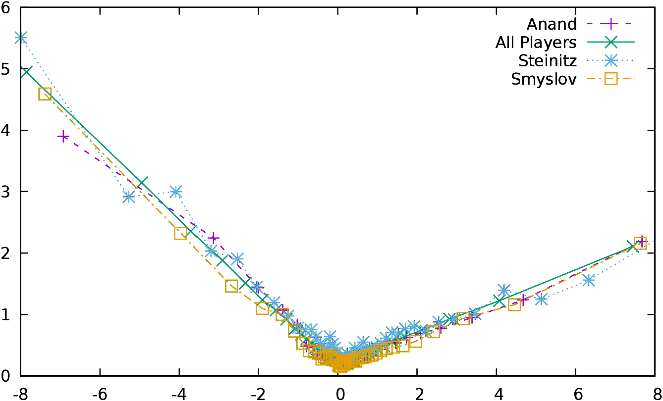
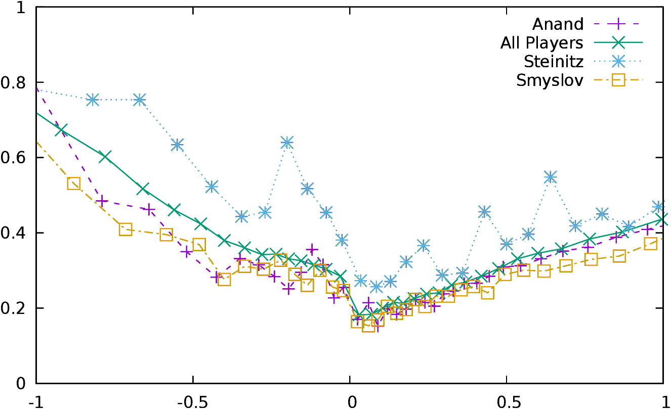
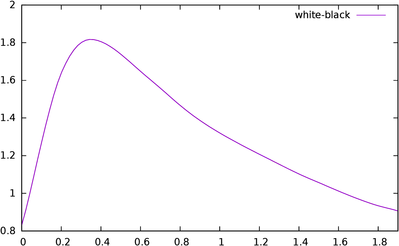
3.2.3 Ponderated conformance
As seen above, Guid and Bratko are performing a “hard cut” at
[−200;200].
We can
see in Figure 2 the distribution of the mean
of the conformance as a function of the evaluation of the
position10. In this analysis, we are only interested in the moves which
have a conformance different from zero, so the latter have been excluded
from the statistics. Moreover, moves have been aggregated in order to
have statistically significant classes (that is the reason why there
are much more points close to 0, one point represents one class).
The curves of all players are extremely similar, and this is
all the most surprising if we consider the “All Players” curve which
represent all the players included in the study, i.e., the World
Champions and their opponents11.
Of course most of the players of this study are world class players,
as World Champions usually do not play against club players, and
the same plot would certainly be different with less strong
players. The slope is not the same if y>0 or if y<0. Players are
making bigger mistakes (that might be seen as “desperate maneuvers”)
when they lose, than
when they win. The relationship is not exactly a linear
one: when we are close to 0 the positive slope is around 0.2,
while it is 0.25 on the whole interval. The difference is even bigger
for the negative slope, with a slope of -0.5 close to 0 and of -0.6 on
the whole interval. However, the average of conformance for a position
with a valuation of y can be approximated
by avg(c(y))=a y + b, with b=0.18, and a=0.26 for y>0 and
b=0.17 and a=−0.60 for y<0 (the values are computed for the
“All Players” curves).
| Figure 2: The distribution of the mean of conformance as a function
of the position evaluation for some selected players. The right
figure is a zoom of the left one.
|
In order to smooth the cut, a ponderated conformance indicator
is defined for each move using the following formula:
if vp is the evaluation of the move played and
vb12
is the evaluation of the best move then
δ=vb−vp is the conformance of the move, and
the ponderated conformance δ′ of the move played is given by:
|
vb ≥ 0 | : | δ/(1+vb/k1) |
|
0 > vb | : | δ/(1+vb/k2)
|
|
The idea is that, while small mistakes made when the evaluation is
already very high (or very low) should count for less, they should not be
completely discarded. The values of k1 and k2 can be chosen using
the results of the statistical analysis above. If we consider that we
map the conformance δ to a new conformance
δ′(vb)=δ(vb)/1+vb/k1
then the average value of δ′(vb) is avg(δ(vb))/1+vb/k1. But
avg(δ(vb)) is also equal to avb+b. Thus
avg(δ′(vb))=a+bvb/1+vb/k1=a1+b/avb/1+vb/k1. This
is equal to a (and is independent of vb) for
k1=a/b. Thus we are going to set k1=0.26/0.18=1.44 and
k2=−0.60/0.17=−3.53.
It is important to stress again why we probably need to ponder δ. The
accumulated conformance indicator method (as well as the distribution
of gain method described in the next section) take as an hypothesis
that an error of δ has the same influence on
the game whatever the evaluation of the position is, and they
“aggregate” all these errors in the same class. This is the debatable point:
making a small mistake in an already won position
seems less decisive than making the same mistake in an equal
position13.
The Markovian interpretation presented in
section 3.4 has been specifically designed to avoid this
pitfall.
In subsection 4.2.2, I experimentally compare and validate
all these indicators by computing their correlation with the outcome of
games using Pearson’s ρ, and
we will indeed see that the correlation with the
outcome of games is better when pondering δ.
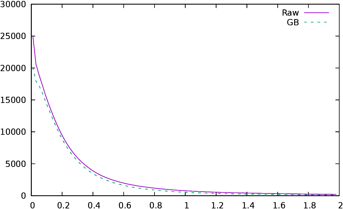
3.3 Distribution of Gain
[Fer12] defines the gain of a move in a way
which is highly similar to the definition of conformance. He computes
the evaluation of the position at game turn k using a fixed depth
search, then at game turn
k+1, and he defines the gain14
as g(k)=vb(k+1)−vb(k). If the position
evaluation made by the computer was perfect, the gain would be
the exact opposite of the raw conformance described above, because the
evaluation at game turn k+1 should exactly be the evaluation of the
move played at position k, and thus
g(k)=vb(k+1)−vb(k)=vp(k)−vb(k)=−δ(k). However, mainly
because of the monotonicity of the evaluation function discussed
above, this is not the case; searching “one move” deeper (because
one move has been made) can often increase the value of the
evaluation, and thus, while δ is always positive, g(k) should
be negative but is not always. Ferreira’s gain method is less “computational
intensive”, as it just requires to compute one evaluation (the
position evaluation) by
game turn, instead of computing two (the evaluation of the best move
and the evaluation of the move played). However, as discussed above;
evaluating two moves instead of one does not multiply the search
time by two, and thus it is better in my opinion to define the gain
exactly as δ (disregarding the sign).
Ferreira does not discuss either the problem of “scaling” (or
pondering) the gain according to the position evaluation (he only
uses “Raw” δ), while it is
exactly the same problem as discussed above regarding conformance.
[Fer12] interprets conformance as a probability
distribution function RP(δ) which represents the probability
for player P to make at each turn a move with conformance δ.
This leads to a different definition of the expected
value of the result of a game between two players. As player one
(p1) and player 2 (p2) have different distribution functions
Rp1 and Rp2, the probability distribution of the difference
between two random variables Rp1 and Rp2 is the
convolution of their distribution Rp1 and Rp2:
|
Rp1−p2(δ)=(Rp2*Rp1)(δ)= | |
Rp2(δ) Rp1(δ+m)
|
Here Rp2−p1=1−Rp1−p2 as it is a probability distribution.
Then Ferreira defines the expected gain for p1 in a game between p1 and
p2 as the scalar product of the distribution vector with
e=(0,⋯,0,0.5,1,⋯,1), as he interprets Rp1−p2(0) as a
draw, Rp1−p2(δ) as a win if δ >0 and as a defeat if
δ<0. Then:
|
s(p1,p2)=0 × | | Rp1−p2(δ) +0.5 ×
Rp1−p2(0) + 1 × | | Rp1−p2(δ)
|
Assuming that the contribution of each element of Rp1−p2(δ)
is the same for all δ< 0 (i.e., 0) and all δ>0 (i.e., 1)
is not obvious.
Using a vector with values starting at
0.0, with a middle value of 0.5 and ending at 1.0, with intermediate
values continuously rising feels more intuitive: the contribution of
Rp1−p2(0.01)
to the expected result “feels” different from the contribution
Rp1−p2(10.00). We will discuss this problem again in
subsection 4.3 when validating experimentally the method.
3.4 A chess game as a Markovian process
The indicators described in sections 3.2 and 3.3
are suffering from the problem described at the end of
subsection 3.2.3.
They basically rely on the idea that an error of δ in a
position P has the same
influence on
the game whatever the evaluation v(P) of the position is, and they
“aggregate” all of them in the same class. Pondering δ is a
way to bend the problem, but the problem is intrinsic to both methods,
and bending it is not solving it. Here, I
am presenting a method which does not rely on this hypothesis.
If the computer program is performing like an
“oracle” always giving the true evaluation of the position and the
best possible move, then the database
gives a way to interpret chess games for a given player as a
Markovian process.
For each position, the computer program is giving us the true evaluation of
the position. This evaluation is assumed to remain constant if the
best available move is played, while it can only decrease if the
player makes a sub-optimal move. The transition matrix, which
is triangular15, gives for each value of the evaluation function the
probability of the value of the evaluation function in the next step.
|
| -1.8 | -1.4 | -1.0 | -0.6 | -0.2 | 0.2 | 0.6 | 1.0 | 1.4 | 1.8 |
|
-1.8 | 1.00 | 0.00 | 0.00 | 0.00 | 0.00 | 0.00 | 0.00 | 0.00 | 0.00 | 0.00 |
|
-1.4 | 0.29 | 0.71 | 0.00 | 0.00 | 0.00 | 0.00 | 0.00 | 0.00 | 0.00 | 0.00 |
|
-1.0 | 0.10 | 0.12 | 0.78 | 0.00 | 0.00 | 0.00 | 0.00 | 0.00 | 0.00 | 0.00 |
|
-0.6 | 0.01 | 0.01 | 0.06 | 0.92 | 0.00 | 0.00 | 0.00 | 0.00 | 0.00 | 0.00 |
|
-0.2 | 0.00 | 0.00 | 0.01 | 0.06 | 0.93 | 0.00 | 0.00 | 0.00 | 0.00 | 0.00 |
|
0.2 | 0.00 | 0.00 | 0.00 | 0.00 | 0.14 | 0.86 | 0.00 | 0.00 | 0.00 | 0.00 |
|
0.6 | 0.00 | 0.00 | 0.00 | 0.00 | 0.04 | 0.14 | 0.82 | 0.00 | 0.00 | 0.00 |
|
1.0 | 0.00 | 0.00 | 0.00 | 0.00 | 0.01 | 0.02 | 0.12 | 0.85 | 0.00 | 0.00 |
|
1.4 | 0.00 | 0.00 | 0.00 | 0.00 | 0.00 | 0.01 | 0.01 | 0.10 | 0.88 | 0.00 |
|
1.8 | 0.00 | 0.00 | 0.00 | 0.00 | 0.00 | 0.00 | 0.00 | 0.01 | 0.03 | 0.96 |
|
|
| Table 2: Transition state matrix for Robert
Fischer in 1971 with g=0.4, binf=−2.0 and bsup=2.0 |
Table 2 presents this matrix computed with all the
games played by Robert
James Fischer in 1971. The rows are the value of the evaluation
function at state t, and the columns are the value of the evaluation
function at state t+1. Each element in the table is the probability
to transition from one state to the other. The sum of all elements in
a line is of course equal to 1, and this table defines a right stochastic
matrix.
For example, regarding state -0.6 (the evaluation function is between -0.4
and -0.8), the
probability to remain in state -0.6 (the evaluation function remains
between -0.4 and -0.8) is 92%, the probability to go to state -1.0
(the evaluation function drops between -0.8 and -1.2) is 6%, the
probability to go to state -1.4 (the evaluation function drops between
-0.2 and -1.6) is 1% and the probability to go to state -1.8 (the
evaluation function drops below -1.6) is also 1%.
State -1.8 is an attractor and can never be left, as the player cannot
enhance his position if his opponent is never making a
mistake. Diagonal values are the higher, as good players are usually
not making mistakes and maintain the value of their evaluation
function.
Building this kind of table depends on three parameters, g
which is the discretization grain, and binf and bsup which
are the bounds outside which a game is supposed to be lost (below
binf) or won (above bsup).
In the previous table, the evaluation function is considered from the
point of view of the player who is going to play, either White and
Black. If
the evaluation function is considered only from White’s point of view, then
two tables are built: one for White and one for Black. White’s
table is the table above; Black’s table is easily deduced from White’s
table using the following formula16,
where n is the size of the matrix
and the array indexes start at 0:
|
MBlack(i,j)=MWhite(n−1−i,n−1−j)
|
|
| -1.8 | -1.4 | -1.0 | -0.6 | -0.2 | 0.2 | 0.6 | 1.0 | 1.4 | 1.8 |
|
-1.8 | 0.95 | 0.03 | 0.01 | 0.01 | 0.00 | 0.00 | 0.00 | 0.00 | 0.00 | 0.00 |
|
-1.4 | 0.00 | 0.77 | 0.11 | 0.04 | 0.00 | 0.08 | 0.00 | 0.00 | 0.00 | 0.00 |
|
-1.0 | 0.00 | 0.00 | 0.78 | 0.15 | 0.07 | 0.00 | 0.00 | 0.00 | 0.00 | 0.01 |
|
-0.6 | 0.00 | 0.00 | 0.00 | 0.78 | 0.17 | 0.05 | 0.00 | 0.00 | 0.00 | 0.00 |
|
-0.2 | 0.00 | 0.00 | 0.00 | 0.00 | 0.79 | 0.20 | 0.01 | 0.00 | 0.00 | 0.00 |
|
0.2 | 0.00 | 0.00 | 0.00 | 0.00 | 0.00 | 0.92 | 0.07 | 0.01 | 0.00 | 0.00 |
|
0.6 | 0.00 | 0.00 | 0.00 | 0.00 | 0.00 | 0.00 | 0.88 | 0.11 | 0.01 | 0.00 |
|
1.0 | 0.00 | 0.00 | 0.00 | 0.00 | 0.00 | 0.00 | 0.00 | 0.80 | 0.12 | 0.08 |
|
1.4 | 0.00 | 0.00 | 0.00 | 0.00 | 0.00 | 0.00 | 0.00 | 0.00 | 0.63 | 0.37 |
|
1.8 | 0.00 | 0.00 | 0.00 | 0.00 | 0.00 | 0.00 | 0.00 | 0.00 | 0.00 | 1.00 |
|
|
| Table 3: Black transition state matrix for Boris
Spassky in 1971 with g=0.4, binf=−2.0 and bsup=2.0 |
White’s matrix is always triangular inferior, and Black’s matrix is
triangular superior. Table 3 is the transition matrix
for Boris Spassky computed from Black’s point of view using all his
games in 1971.
Now if Fw is Fischer’s (White) matrix and Sb Spassky’s
(Black) matrix the product:
is the matrix holding the transition probabilities after a sequence of
one white move and one black move
(probability vectors v are row vectors and will be
multiplied from the left, such as in v MFw,Sb = (v Fw) Sb,
using the convention of right stochastic
matrices).
M is also a stochastic matrix, as
it is the product of two stochastic matrices. As such, there exists a
vector π which is the limit of:
One of the properties of the limit π is that it is independent of
π0 as long as π0 is a stochastic vector (the sum of all
elements of π0 is 1), and that it is itself a stochastic vector,
called the stationary state of the Markov chain. Instead of calculating
the limit, this vector
can be easily computed by finding the only stochastic eigenvector
associated to eigenvalue 1.
Using 1971 data from Fischer and
Spassky, the stationary vector is:
|
π=(0.07,0.01,0.01,0.04,0.14,0.18,0.07,0.04,0.04,0.40)
|
The (very) rough interpretation is that the outcome of a match between
them should have been
40% wins for Fischer, 7% wins for
Spassky and 53% of games drawn17.
The 1972 World Championship, if
Fischer’s forfeit in game 2 is removed, ended in +7=11-2, or 35% wins
for Fischer, 10% wins for Spassky and 55% of games drawn18.
4 Fitting, validating, comparing
In section 4.1 I am quickly dealing with the complexity indicators
presented in the literature and in websites.
These indicators, while
interesting, are not as “rich” as the cumulative conformance
(4.2), the covariance (4.3) and
the Markovian (4.4) indicators;
the methodology for these three indicators will mainly be the same: I
first check on individual games that the indicator has a
good correlation with the outcome of the game, and we try to enhance
this correlation by fitting the model to the data. Then I evaluate the indicator
not on one game, but on a set of games (here World Championships) to
see if “averaging” it on a more macroscopic scale gives coherent results.
Then, I compare it to the ELO ranking system,
regarding its ability to predict the outcome of games and to rank
players.
Last I evaluate how they can be
used to rank players (which is simple for the accumulated conformance
indicator, but not so simple for the other two).
To do this, I am going to use the World Championships for which
the complete data for the two players are available19, and I am
going to compute the three indicators for the year just before the
championship, using a “forgetting factor” as described in
section 3.2. I will then use these indicators to
compute the predicted result of the championship, and I will compare it
to the actual result and to the predicted outcome compute with the ELO
model (when ELO rankings exist).
A quick reminder might be useful here;
the ELO ranking system was designed, from the start, to be able to
estimate the probability of the outcome of a game between two players,
and in this system estimating the outcome and ranking players is
intimately linked as they both depend on each other: points are
added (respectively subtracted) when you defeat a player who has a better
ranking (respectively when you lose against a player with a lesser ranking),
and the rankings are used to estimate the expected outcome of a game.
There is no such relationship for intrinsic indicators.
One advantage of the intrinsic predictors is that, as soon as they
have been computed, they enable to compare any players even if they
belong to completely different periods.
They are only based on the conformance of moves
(the “quality of play” is intrinsic to a player) and are thus
completely independent of the possible “drifting through years”
problem of the ELO indicator.
4.1 Complexity indicators
I present in Table 4 the
correlations between the magnitude of the error made by the player
with the following indicators.
-
D/t:
- Depth vs Time: describes complexity as a function of the
depth reached regarding time use to reach it.
- Stab:
- Stability: depends on the mean delta in the evaluation
function between two consecutive depths in the search (see
section 3.1).
- JumpV:
- Jump Value: depends on the largest difference in the
evaluation function between
two successive depths in the search.
- JumpD:
- Jump Depth: depends on the depth where the difference
between two successive evaluations are the largest.
- JD x JV:
- Jump Depth times Jump Value: product of the previous
two indicators.
(see section 3.1).
The correlations were computed using Pearson’s ρ20.
These indicators were computed for all the moves played by each World
Champion, and were also aggregated for all moves played by all World Chess
Champions (the Champs line). They were also computed for all the
moves of all the games present in the database (the All
line). The Others line is the complement of the All line
and the Champs line (i.e., all moves present in the database
played by players who were not World Champions).
|
Name | D/t | Stab | JumpV | JumpD | JD x JV |
|
Steinitz | 0.092 | 0.327 | 0.349 | 0.176 | 0.361 |
|
Lasker | 0.046 | 0.235 | 0.296 | 0.147 | 0.306 |
|
Capablanca | 0.081 | 0.355 | 0.417 | 0.149 | 0.432 |
|
Alekhine | 0.064 | 0.282 | 0.315 | 0.185 | 0.343 |
|
Euwe | 0.046 | 0.220 | 0.306 | 0.141 | 0.311 |
|
Botvinnik | 0.071 | 0.333 | 0.427 | 0.128 | 0.439 |
|
Smyslov | 0.035 | 0.189 | 0.233 | 0.123 | 0.223 |
|
Tal | 0.058 | 0.256 | 0.311 | 0.129 | 0.290 |
|
Petrosian | 0.044 | 0.241 | 0.285 | 0.110 | 0.300 |
|
Spassky | 0.044 | 0.270 | 0.301 | 0.136 | 0.314 |
|
Fischer | 0.011 | 0.273 | 0.310 | 0.134 | 0.313 |
|
Karpov | 0.046 | 0.216 | 0.264 | 0.122 | 0.270 |
|
Kasparov | 0.058 | 0.313 | 0.384 | 0.128 | 0.385 |
|
Khalifman | 0.074 | 0.258 | 0.317 | 0.138 | 0.347 |
|
Anand | 0.057 | 0.243 | 0.329 | 0.131 | 0.344 |
|
Ponomariov | 0.048 | 0.156 | 0.174 | 0.150 | 0.168 |
|
Kasimdzhanov | 0.056 | 0.340 | 0.405 | 0.106 | 0.350 |
|
Topalov | 0.036 | 0.223 | 0.252 | 0.135 | 0.276 |
|
Kramnik | 0.056 | 0.253 | 0.290 | 0.148 | 0.307 |
|
Carlsen | 0.061 | 0.252 | 0.319 | 0.125 | 0.295 |
|
Champs | 0.053 | 0.254 | 0.308 | 0.135 | 0.312 |
|
Others | 0.031 | 0.104 | 0.104 | 0.138 | 0.101 |
|
All | 0.038 | 0.161 | 0.185 | 0.135 | 0.180 |
|
|
| Table 4: Correlations of complexity indicators: Depth vs time, Stability, Jump Value, Jump Depth and a composite of Jump Value and Jump Depth |
The first thing to notice is the fact that the D/t indicator is almost
not significant. The correlation is extremely low, even if it is
always positive, for all players. Apparently, the branching factor of the
tree does not seem to be a very good indicator of what some authors
call “the complexity” of the
position. However, there is no indicator which is extremely
significant. The best one seems to be the composite JumpxDepth
indicator, which is equal to 0.312 for World Champions, while it is
only 0.101 for the other players. The most plausible interpretation is
that World Champions usually play the “right moves” when the
positions are stable, and make mostly mistakes in unstable positions,
while “ordinary” players are more prone to make mistakes in all
kind of positions. The only players having an indicator over 0.4 are
Botvinnik and Capablanca, which were famous for their positional and
consistent play.
A lesson to learn from these indicators is probably that on the one
hand, it would be interesting to collect and save more data during the
search, such as the value of the evaluation for all depths of the
search (and not only the mean and the max), to try to compute other
indicators, as the ones computed here, while interesting, do not seem
to carry an extremely high significance. On the other hand, it is also
possible that there is no such thing as a simple “complexity
indicator” of a position that could be correlated with the errors
made by the players, and that the complexity of the position depends
on many other, less evident, factors.
4.2 Cumulative Conformance
The cumulative conformance section is partitioned into four
subsections: correlation with the outcome of a game
(4.2.1), conformance of play in World Championships
(4.2.2), conformance of play during a whole career
(4.2.3) and predicting the results of World Championships
matches (4.2.4).
4.2.1 Correlation between cumulative conformance
and the outcome of one game
In section 3.2 I have defined different possible indicators regarding the
conformance of moves. Below, I am going to correlate these indicators
to the outcome of games using again Pearson’s ρ.
| Figure 3: Distribution of conformance, excluding first and last
class |
First, it is interesting to have an idea of the distribution of the
conformance for all the positions evaluated during this study. We only
keep positions after game turn 10 and positions where the move
to play is not forced. This leaves around 1,600,000 positions
(respectively 1,350,000 for Guid and Bratko who eliminate positions
with an evaluation lower than -2.00 or higher than 2.00). The
conformance is equal to 0 for 980,000 moves (respectively 842,000), which is
a large
majority. In Figure 3 the number of positions for
each conformance, up to 1.99, is plotted (conformance is measured in
centipawns, so it starts at 0.01 and goes up to 1.99 by 0.01
steps). The class after 1.99, which is not plotted, contains all
positions with a conformance greater than 2.00; there are around 53000
such positions.
For each game and each type of conformance,
three different kinds of conformance (as
defined in section 3.2) are computed. We quickly summarize them below.
-
Raw conformance δ=vb−vp is just the raw difference between
the evaluation vb
of the best move and the evaluation vp of the move made by the player.
- Guid and Bratko conformance is defined in a similar way, but
the positions with an evaluation higher than +2 or lower than -2 are
not considered.
- Ponderated conformance is defined by δ′=δ/(1+vb/k1) for
vb>0 and δ′=δ/(1+vb/k2) for vb<0, where k1
and k2 are
suitable constants. In subsection 3.2.3, after a
statistical analysis of the distribution of errors,
k1=1.44 and k2=−3.53 are chosen.
In the rest of this section, each time the word “conformance” is
used, it can represent any of these three meanings, except when
explicitly stated otherwise.
We are interested in the cumulative conformance for White
(respectively Black) during one game defined by pw(x) (respectively pb(x)):
|
pw(x) | = | |
| | nb_moves_white(δ≤ x) |
|
| total_moves_white |
|
|
|
pb(x) | = | |
| | nb_moves_black(δ≤ x) |
|
| total_moves_black |
|
|
|
total_moves_white
(respectively Black)
is the total number of white moves in the game which are taken
into account: this value is simply the number of white moves in this game
minus the opening moves and minus the moves which are
forced (there is only one move possible)21.
nb_moves_white(δ≤ x) (respectively Black) is the number of moves
with a conformance less than or equal to x, taken only in the moves
taken into account as defined above.
Then p(x)=pw(x)−pb(x) is the difference between
White’s and Black’s conformance for a given game. There are around 26,000 games, and
thus 26,000 p(x) for each x. Now, we wish to know for which value of x
p(x) has the best correlation with the outcome of the game. Thus, for
each x we compute Pearson’s ρ by correlating for each x the
26,000 p(x)
with the outcome of the 26,000 corresponding games (+1 if White wins, 0
for a draw and -1 if White loses).
An optimization was quickly performed using a
[NM65]
simplex algorithm22
to find the best correlation possible, and the optimal values found are
k1=0.75 and k2=−3.3.
Figure 4 represents the correlations of the accumulated
conformance indicators starting at conformance 0.
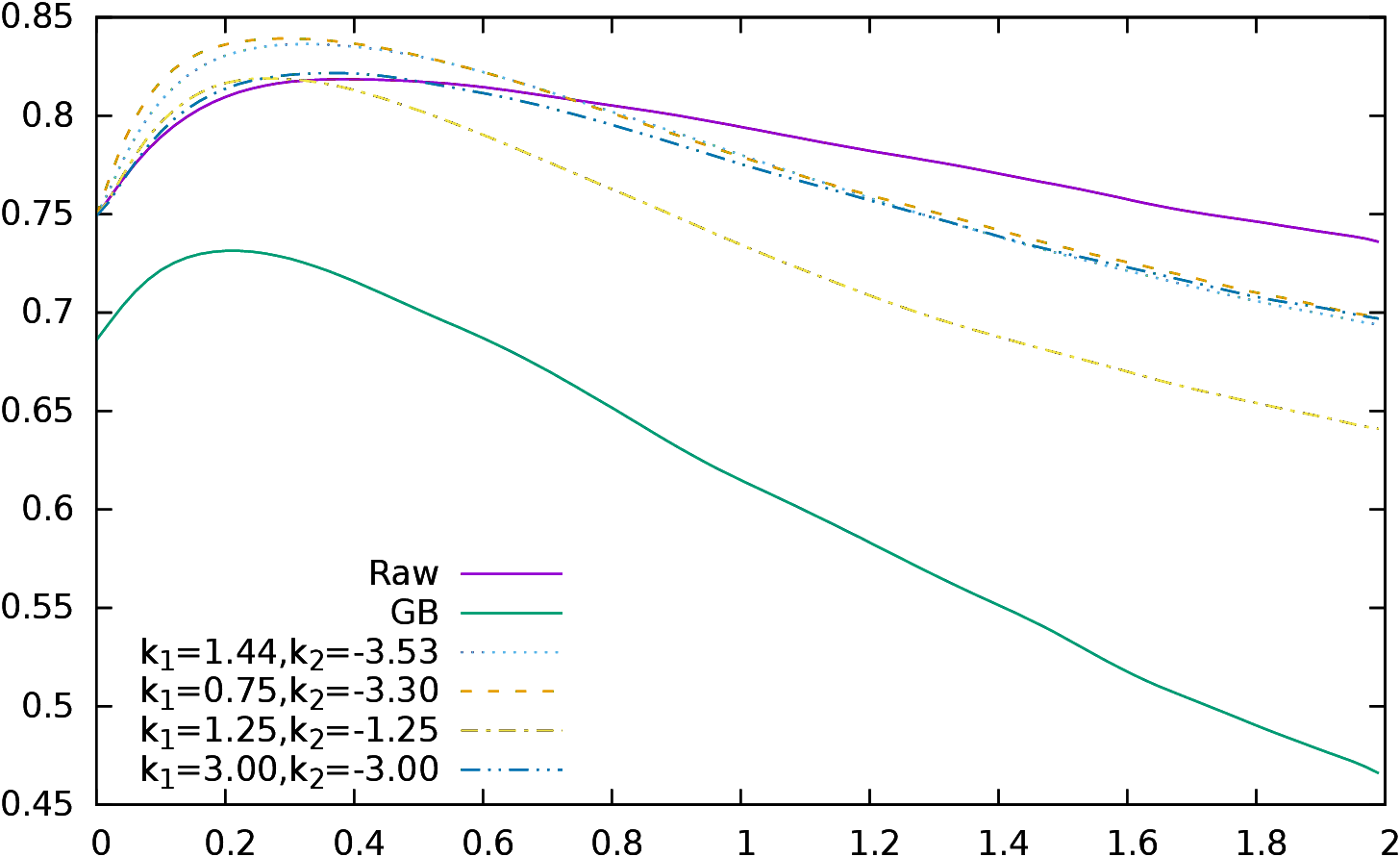
| Figure 4: Correlation of accumulated conformance indicators for raw
conformance, G&B conformance and different values of k1 and
k2 for ponderated conformance. |
The best correlation is
found for d≤ 0.3 for the raw and ponderated conformances, and for
d≤ 0.2 for the G&B conformance. It is interesting to notice that
the choices made for k1=1.44 and k2=−3.53 in
subsection 3.2.3 work
remarkably well when compared to the optimal curve k1=0.75 and
k2=−3.30. The decision to use two different slopes depending on the
sign of the evaluation function is also validated when we compare the
previous curves to the curves defined by k1=−k2=1.25 and
k1=−k2=3.00.
It is important to try to understand why there is a
“bump” in the curve representing correlation (i.e., why the optimal
correlation is reached around δ≤ 0.30 and not somewhere else). My
interpretation is the following: having a better conformance
for “perfect” (d=0) moves is of course extremely
important because the “perfect” moves class is by far the largest
and overshadows the others. However, having a better conformance here
does not tell us anything about the distribution of the other moves,
and even if there are less moves in the other classes, there are still
some of them, especially in the class closest to 0. Thus “adding”
those classes to the conformance indicator gives more information
about the distribution of the moves and “captures” important
information. However, after a point, adding new classes which
contain a small number of moves adds less meaningful information, and
the correlation decreases.
There is still an other point to discuss: how is the outcome of the game
correlated to the mistakes made, in other words what happens when we
correlate the outcome of the game to p′(x) defined by
|
pw′(x) | = | |
| | nb_moves_white(δ≥ x) |
|
| total_moves_white |
|
|
|
pb′(x) | = | |
| | nb_moves_black(δ≥ x) |
|
| total_moves_black |
|
|
|
p′(x) | = | pw′(x)−pb′(x)
|
|
First, let us notice that
nb_moves_white(δ≥ x)+nb_moves_white(δ≤
x)=total_moves_white. So:
|
pw′(x) | = | | nb_moves_white(δ≥ x) |
|
| total_moves_white |
|
| | = | | total_moves_white−nb_moves_white(δ≤
x) |
|
| total_moves_white |
|
| | = | | 1− | | nb_moves_white(δ≤ x) |
|
| total_moves_white |
|
|
| | = | 1−pw(x)
|
|
Thus Pearson’s ρ for p′(x) is23 −ρ(p(x)). Thus the curve representing the correlation of
p′(x) will be exactly the opposite of the one of p(x), with the
same extrema at the same positions.
This result might seem paradoxical. Intuitively, we might think that
making big errors should be quite strongly correlated to the result of
the game. This is of course true: in Figure 13
in subsection 4.4.1
we will see that
the result of the game is very strongly correlated to the highest
evaluation reached in the game. But here
the accumulated conformance indicator(s) is not measuring this kind of
correlation. Accumulated conformance is in fact measuring the
combination of two things at the same time: on the one hand, it has to
take into account how often a player is losing a game when
he24 is
making a (big) mistake, but it also depends on the probability of
making big mistakes. A player who loses always when making a 50cp
mistake, but only makes such mistakes one game out of one hundred will
lose less often than a player who never loses games when he makes a
50cp error, and loses them only when he makes a 100cp error, but
makes such mistakes one game out of fifty.
It is important to remember that I have only be maximizing the
correlation of the difference of the accumulated conformance indicator
with the result of the game, which is not the same thing as “fitting” the
value of the difference of the conformance between two players with
the result of the game. As Pearson’s ρ is invariant under
linear scaling, it is possible using a classical least square
method to find α and β such as r=β d +
α is the best approximation of the actual result of the game
(here d stands for the difference of the conformance indicators of the two
players). This will of course not change Pearson’s ρ, so this
computation can be done independently of the optimization of k1 and
k2, and we can compute α and β for all possible values
of x such as δ ≤ x. We expect25α to be rather close to 0,
while β should increase with x.
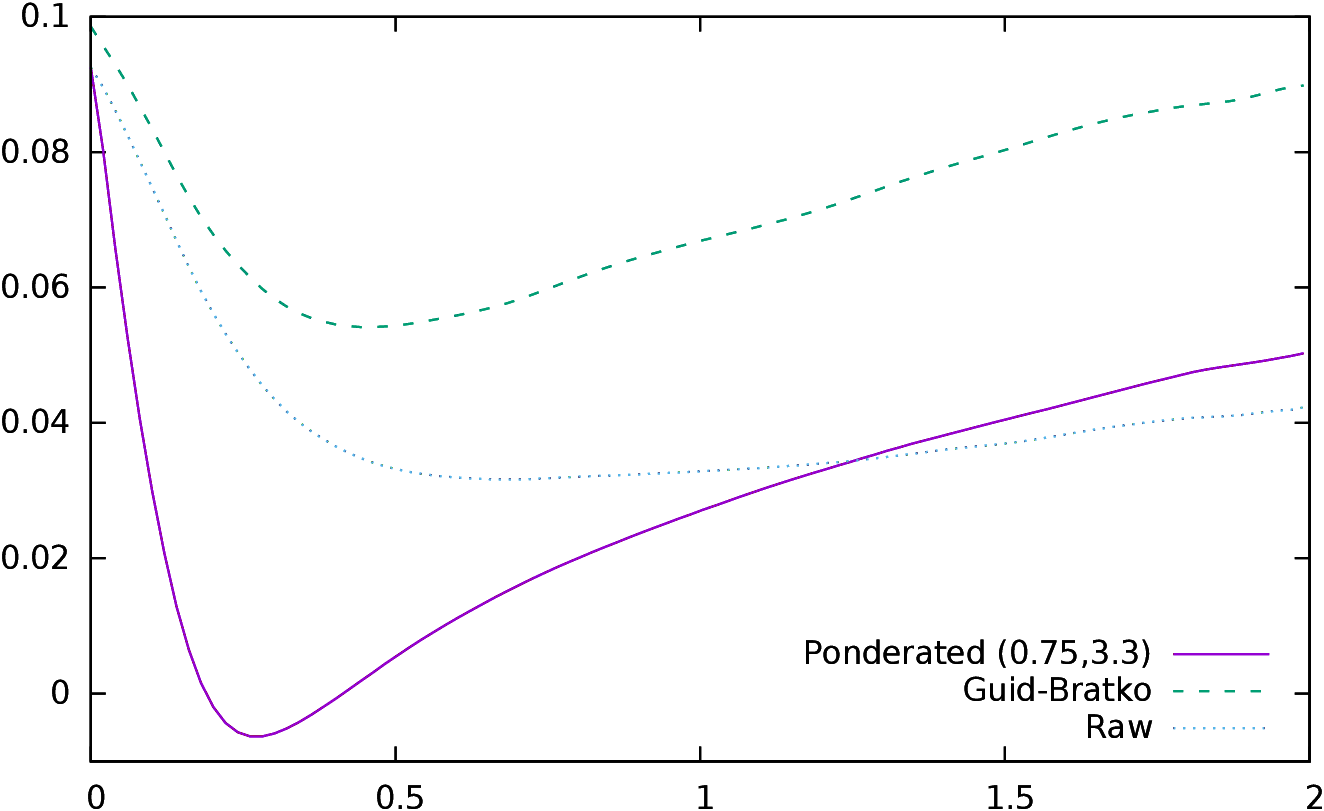
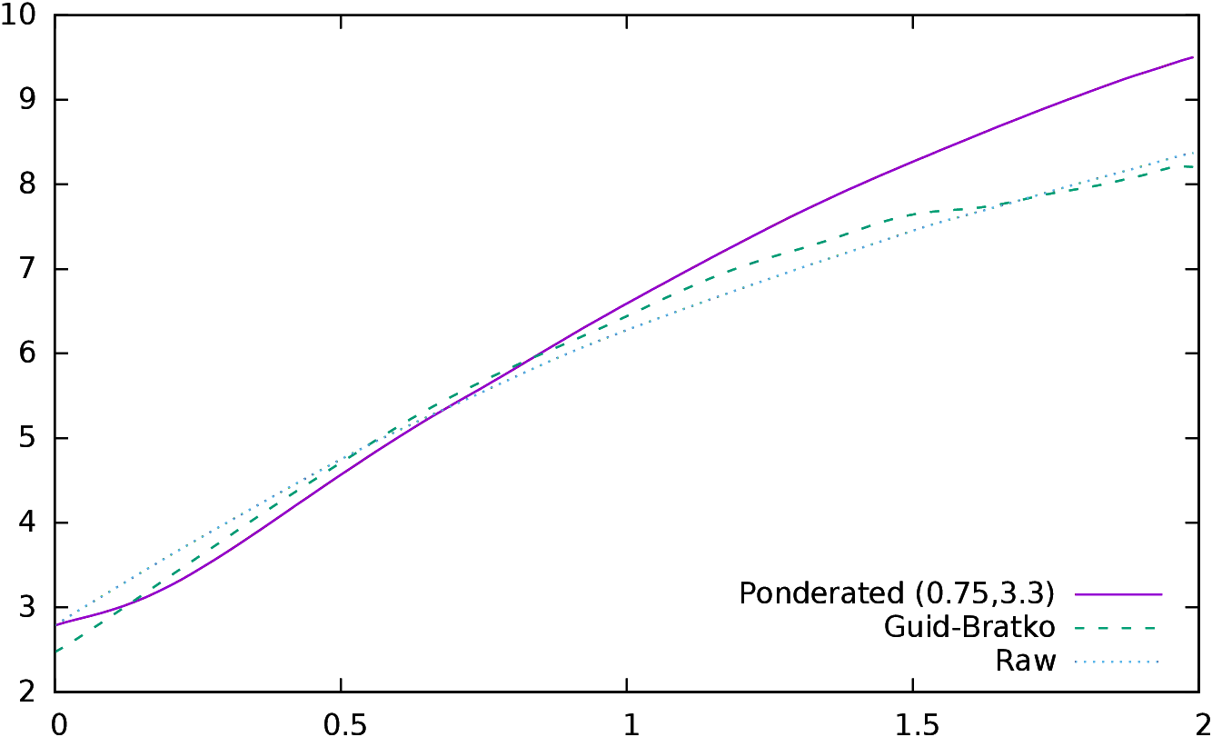
| Figure 5:
α (left) and β (right) values as a function of the
difference of the accumulated conformance indicators of the two players.
|
In Figure 5 we have plotted the values of β and
α as a function of x. Let us remember that the optimal value
of x is 0.3 for
ponderated and raw conformance, and 0.2 for Guid and Bratko
conformance; the optimal values of (α,β) are: Raw
(α=4.3 10−2, β=4.00), Guid and Bratko
(α=6.7 10−2, β=3.37), and Ponderated (α=−7.0 10−3,
β=3.64).
The values of α show that there is a small
positive bias regarding raw conformance (and Guid and Bratko
conformance). The correlation has always been computed by
subtracting Black’s
value from White’s value, so this shows that,
for identical raw values of the
conformance indicator, White wins more often than Black26.
A quick statistical analysis of the 26,000 games shows that
the average score of a game is 0.12 (White is winning 56% of the
points). It is common knowledge that, in chess, White wins slightly more often
than Black, and the usual
explanation is that White’s positions are usually “better” as White
plays first. This explanation is of course correct27, but
there might be another factor.
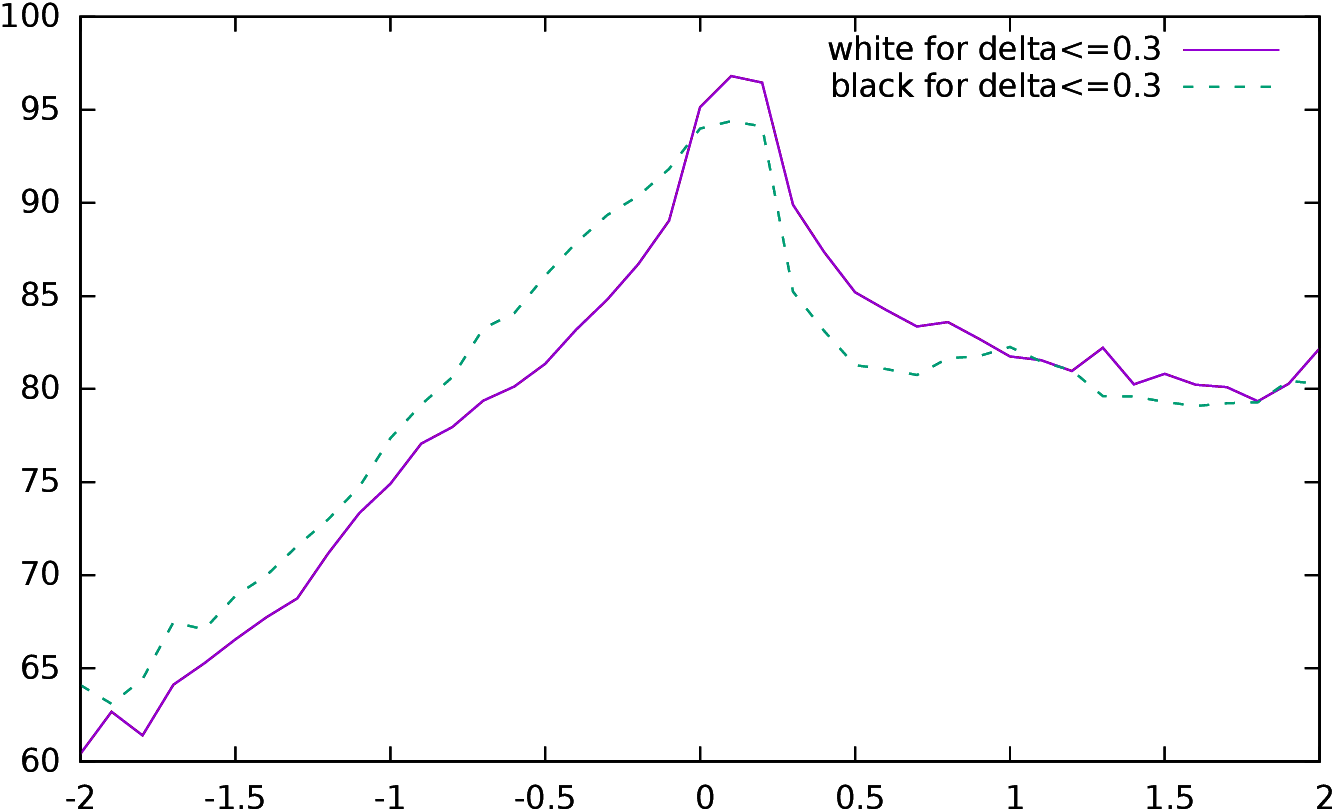
| Figure 6:
Difference between the accumulated raw conformance indicator of White
and Black (in percent) as a function of δ (left), and
percentage of moves with an accumulated raw conformance δ≤
0.3 as a function of the position evaluation (right)
|
When plotting the difference of the raw accumulated
conformance indicator for White and for Black, it is always
positive (see left part of Figure 6). White
is playing 61.1% perfect moves (x=0),
while Black is only playing 60.2% perfect moves. The difference
even rises for larger x and is maximal around x=0.25 where it
reaches almost 2%. So, Black is in a way, making more mistakes than
White. Why it is so is more difficult to interpret. We have already
seen (subsection 3.2.3) that players are making more serious
mistakes when they are in
unfavorable positions; as Black is usually starting with a slight
disadvantage, the same kind of psychological bias might encourage them
to take more risks, and thus to make more mistakes.
On the right side of Figure 6, we see
that the distributions of White’s and Black’s conformance are
different. White is performing better at 0 and slightly above, while
Black is better below 0. This figure also confirms that while the
level of play remains consistent when the evaluation of the position is
positive, it is degrading fast for negative ones.
We also understand why ponderated conformance corrects the bias: it is
“stretching” differently the positive and the negative side of the
curve because it is using two different constants to “bend” the
distributions.
The fact that the difference between White and Black is maximal around
x=0.25 might be another reason why the accumulated conformance
indicator has the best correlation around this value.
In conclusion, the advantage of the accumulated conformance indicator
is that it is a
scalar, and it is thus easy to consider it as a ranking. The player
with the best indicator is just supposed to be the best
player. However, this discussion should remind us that cumulative conformance is
not a beast which is easily tamed, and it is much more difficult to
interpret it than it might seem at first glance. A second important thing
to remember is that we have “fitted” the model to the data using
only games played by world class champions; it is extremely possible
that results and parameters would be different for club players, as
the distribution of their moves is very different; thus some classes
with high δ which are marginal here could have a much higher
importance.
4.2.2 Conformance of play in World Championships
In this subsection we are working on many
games at once. The conformance is computed for all the moves
in all these games at the same time;
we are using here
World Championships games, in the same way as
the previous work by Guid and Bratko concentrated exclusively on
these games.
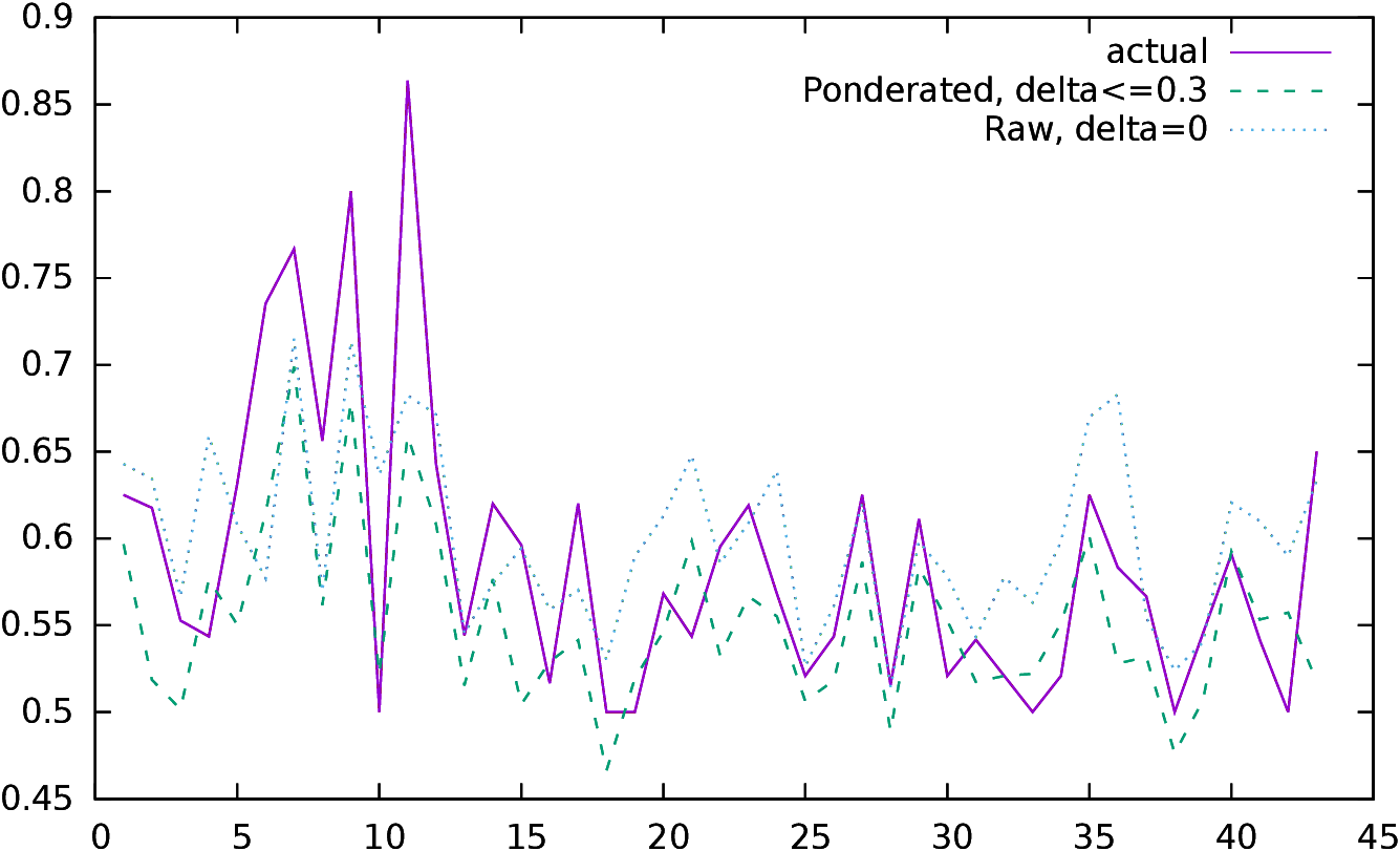
The left part of Figure 7 gives for each championship
since 1886 (1) the actual result, (2) the expected result using the
accumulated conformance indicator and (3) the expected result using
simply the percentage of “perfect moves” (appropriate α and
β as defined in the section above are used to scale properly the
indicator).
The number of games, or the time controls were not identical
for all these events, but they were mainly similar. The
results for the FIDE World Championships played in k.o. mode from
1998 to 2004 are not taken into account, as these time controls were
criticized for lowering the quality of play.
| Figure 7:
Actual score and expected scores for all World Championships
since 1886 (left) and difference of conformance between two
opponents for four World Championships.
|
The correlation of the actual result with the indicators
is adequate, but visually it is not so clear that the ponderated
conformance is much better than the simple “perfect move” percentage.
The ponderated conformance is usually closer to the actual result,
which is often overestimated by the “perfect move”
percentage. However, the ponderated conformance
sometimes “misses” results, such as the result of the last WCH
(Carlsen-Anand 2013), which is grossly underestimated.
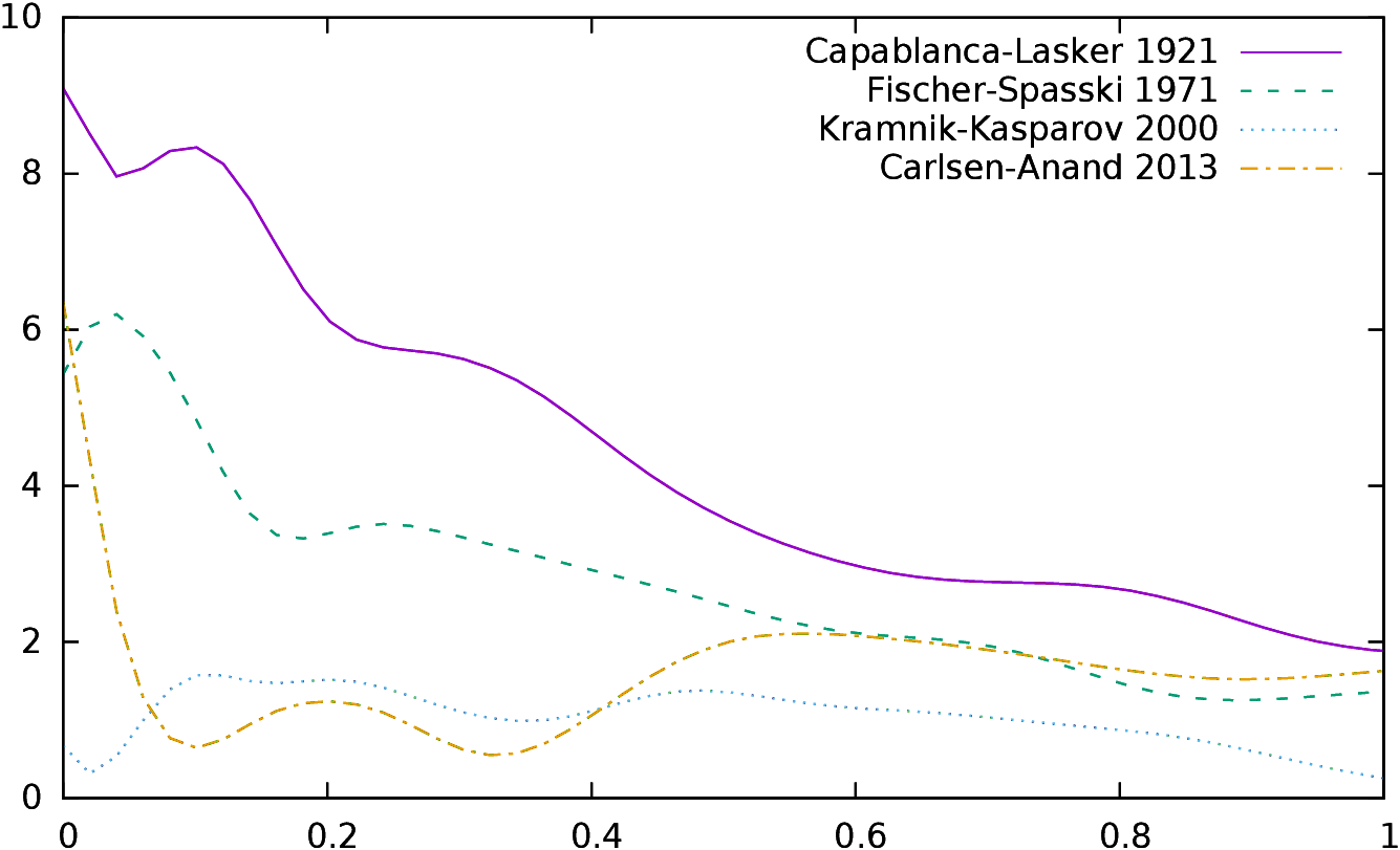
In the right part of Figure 7, we plot the difference in
conformance between the two opponents for four World
Championships28.
This curve tells us why ponderated conformance at δ≤ 0.3 is
partly missing its target for the 2013 Championship.
The difference between Carlsen and Anand is
extremely high for δ=0 and then falls steeply, and is small
around δ≤ 0.3. A careful visual study of all the curves for
the 41 World Championship hints to a possible interpretation; it looks
like the result depends first on the difference of the
indicator for δ=0. However, if this difference becomes “small”,
then the result seems to be determined by the difference for higher
values of δ. This remark has to be taken with extreme caution and
requires further investigation, but it is not impossible, as this
indicator is an aggregator, and its interpretation is complex.
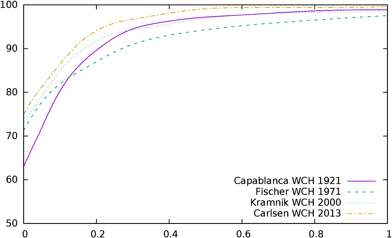
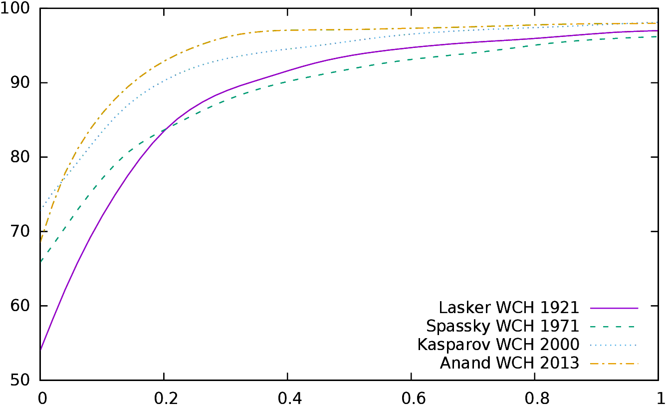
| Figure 8:
Performance of winners (left) and losers (right) in four World Championships
|
In Figure 8 we plot the performance of winners (left)
and losers (right) during these four WCH.
The performance by José Raul Capablanca in 1921
is definitely remarkable29: 63% of
his moves were exactly those chosen by the computer (0cp), 81% were
at a score less than 10cp of
the move chosen,
90% at a score less than 20cp and 95% at a score less than 30cp. It took
years to
find other players able to perform so well in a WCH.
It is however interesting to
notice that the “conformance” of players has steadily raised. In 2013,
Magnus Carlsen scored respectively 75% at 0cp, 86% at 10cp, 95%
at 20cp and 97% at 30cp. For all championships from 2000 to 2013, all
winners scored
better than Capablanca at 0cp, and most of them scored better at 10cp,
20cp and 30cp. Kasparov lost the 2000 WCH while his performance was his
best ever in a WCH, Kramnik was simply better.
4.2.3 Whole career
Figures 16 and 17
display the conformance indicator for all World Champions for their
whole career, respectively for d=0 (Fig. 16)
and d≤ 0.3 (Fig. 17).
Players perform differently depending on the bound set on move
conformance. For example, Fischer has outstanding records for d=0,
while his performances for d≤ 0.3 are more ordinary30.
4.2.4 Predicting the results of World Championships
Below we compare the score predicted for World Championships by
the accumulated conformance predictor (Acs) to (1) the actual score
(As) and to (2) the
score predicted
using ELO tables (ELOs). This indicator can only be computed
for the World Championships where both players were at least
once World Champion, because only World Champions have all their games
evaluated.
The available results are presented in Table 5 in the
Acs column. Column As contains the actual score of the WCH and
ELOs the predicted result of the championship according to the ELO ranking
of both players when it was available (column Covs contains
covariance predicted score and column Ms Markovian predicted scores,
see subsections 4.3.3 and 4.4.3). The
accumulated conformance
predictor Acs is computed by taking the result of the games played by both
players the year before the WCH and applying the parameters giving the
best correlation (δ=0.3, α=−0.007, β=3.64,
k1=0.75, k2=3.3).
|
Championship | Acs | Covs | MS | AS | ELOS |
|
Euwe-Alekhine 1935 | 57% | 60% | 61% | 52% | |
|
Alekhine-Euwe 1937 | 53% | 51% | 57% | 62% | |
|
Smyslov-Botvinnik 1957 | 50% | 49% | 51% | 56% | |
|
Botvinnik-Smyslov 1958 | 45% | 48% | 49% | 54% | |
|
Botvinnik-Tal 1961 | 49% | 51% | 52% | 59% | |
|
Petrosian-Botvinnik 1963 | 51% | 58% | 57% | 57% | |
|
Petrosian(2660)-Spassky(2670) 1966 | 49% | 65% | 45% | 52% | 48% |
|
Spassky(2690)-Petrosian(2650) 1969 | 48% | 33% | 54% | 54% | 56% |
|
Fischer(2785)-Spassky(2660) 1972 | 54% | 53% | 63% | 63% | 67% |
|
Kasparov(2710)-Karpov(2700) 1985 | 47% | 46% | 53% | 54% | 51% |
|
Kasparov(2710)-Karpov(2700) 1986 | 50% | 51% | 51% | 53% | 51% |
|
Kasparov(2720)-Karpov(2720) 1987 | 48% | 48% | 48% | 50% | 50% |
|
Kasparov(2770)-Karpov(2710) 1990 | 53% | 55% | 54% | 52% | 59% |
|
Kasparov(2820)-Anand(2720) 1995 | 51% | 54% | 50% | 58% | 64% |
|
Kramnik(2730)-Kasparov(2810) 2000 | 51% | 48% | 59% | 57% | 39% |
|
Anand(2800)-Kramnik(2785) 2008 | 50% | 42% | 52% | 54% | 52% |
|
Carlsen(2840)-Anand(2780) 2013 | 54% | 54% | 60% | 65% | 58% |
|
|
| Table 5: Accumulated conformance predicted score (Acs),
Covariance predicted score (Covs), Markovian predicted scores
(MS), actual scores (AS) and ELO predicted scores (ELOS)
when available for World Championships |
For the 11 World Championships for which the ELO prediction is available,
the mean difference between the actual score and the ELO predicted
score is 5%. For the accumulated conformance predictor, the mean
difference between the actual score and the accumulated conformance
predicted score is 6% on all championships and of 5% on the 11 World
Championships for which the ELO predictor is available. So, the
accumulated conformance predictor is giving on the whole good results,
on par with the ELO predictor. We will further discuss this predictor
when we will compare the three predictors.
4.3 Gain and distribution covariance
The gain and distribution covariance section is partitioned into three
subsections: correlation with the outcome of a game
(4.3.1), conformance of
play during a whole career (4.3.2), and predicting the
results of World
Championship matches (4.3.3).
4.3.1 Correlation with the outcome of a game
In this subsection we are going to see how computing the expected result
of a game by using Ferreira’s distribution method
(presented in section 3.3)
fares. Thus, for each game, I compute the vectors RW(δ) and
RB(δ) of the
distribution of δ for each player for the given game,
and the convolution of the two distributions, which gives us the
distribution of RW−B.
Then I compute the scalar product of this vector with the vector
describing the expected gain, which is in Ferreira’s paper
e=(0,⋯,0,0.5,1,⋯,1). The
result should be the expected outcome of the given game.
The first goal here is thus to evaluate the correlation of this covariance
indicator with the outcome of the games, as we did in
subsection 4.2.1 for the accumulated conformance
indicator. It can be done for raw δ (that is what Ferreira is
doing in its paper), but it can also be extended to G&B
conformance and to ponderated “bi-linear” conformance. Results are
available in Table 6, where (k1=1.44,k2=−3.53) are
the values found in subsection 3.2.3 through linear regression
and (k1=0.37,k2=−3.70) are the optimal values found when optimizing
the values of k1 and k2 with, here again, a Nelder-Mead simplex
to get the best possible correlation.
|
| Raw | G&B | k1=1.44 | k1=0.37 | k1=1.20 | k1=0.82 |
|
| | | k2=−3.53 | k2=−3.70 | k2=−3.41 | k2=−2.37 |
|
| | | | | s=1.16 | Spline |
|
ρ | 0.806 | 0.749 | 0.817 | 0.825 | 0.875 | 0.879 |
|
x | 0.012 | 0.010 | 0.018 | 0.031 | 0.020 | 0.017 |
|
σx | 0.225 | 0.227 | 0.240 | 0.263 | 0.132 | 0.103 |
|
β | 2.682 | 2.460 | 2.553 | 2.346 | 4.956 | 6.420 |
|
α | 0.082 | 0.089 | 0.067 | 0.041 | 0.014 | 0.012 |
|
|
| Table 6: Statistical results for the covariance
indicator |
The table also holds the mean (x) of the estimated result (values are
in [−1,1]), its standard deviation (σx), and the values of
β and α which have been computed in exactly the same way
as in the previous section. The mean of the actual game outcomes is
0.12 (56% for White) and the standard deviation is 0.75.
We can deduce a plethora of things from these results. First, while the mean
is approximately correct (it is almost 0, with a slight bias for
White, as in the previous section), the standard deviation is much too
small. This was not much of a concern regarding the accumulated
conformance indicator in the previous section, which did not claim to
represent the actual outcome of the game, but it is here a hint that
something is not correct, as the interpretation of the scalar product
of the covariance vector with the gain vector e was supposed to be an
estimation of the outcome of the games, and not to be only correlated with
it. Thus, we have to apply a linear scaling function, with
coefficients β and α which are quite similar to the ones
found for the accumulated conformance indicator in the previous section.
Second, the best optimal correlation found (0.825 for ponderated
conformance) is less than
the best correlation found in section 4.2 for the
optimal accumulated conformance indicator. We should have expected the
opposite: the accumulated conformance indicator is a scalar value, and
thus captures less information than this indicator, which “represents”
a player’s style by a vector instead of a scalar.
The first thing to do is to seriously
reconsider the values of vector e. As a quick experiment, we set
coefficients in e according to the function:
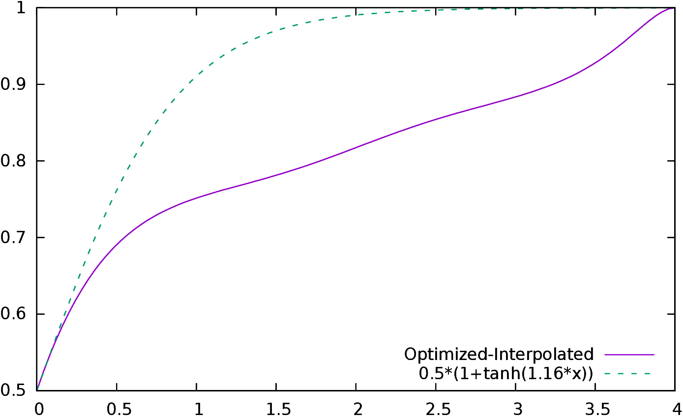
| Figure 9: Values of the coefficients of vector e as a function of
the difference of the two random variables |
Here, a is a suitable constant to determine. Using again a Nelder-Mead
optimization but on three parameters (k1, k2 and a), we find the
optimal values
k1=1.20, k2=−3.41 and a=1.16 with an optimal correlation of
0.875, which is this time better than the one found for the
best accumulated conformance indicator.
In Figure 9, we have
the curve describing the shape of the coefficients of vector e.
In order to validate these coefficients, a second optimization was
performed, on 21 variables, two for k1 and k2 and 19 for fitting
19 points of a spline. Coefficients were set to 0.5 at 0 and to 1.0
at +4, and the 19 variables gave the value of the coefficient at
(0.2,0.4,⋯,3.6,3.8). The other values were interpolated. The
shape of the curve is quite different, however the correlation is only
slightly better (0.879), and the
mean, the standard deviation, α and β are
similar (β is even higher). This means that, on the one hand,
the correlation is not very
sensitive to the parameters, and on the other hand that this indicator
also needs to be “stretched” in order to predict the scores, just
like the conformance indicator.
This is not really surprising.
I have here mainly followed Ferreira’s presentation and
interpretation found in [Fer12]. In the paper, Ferreira links
directly the distribution Rp1−p2 to the expected score of the
game by the formula presented also here in
section 3.3. This is however a little
far-fetched. Rp1−p2(x) is the probability that the score
evolves by x after a sequence of two moves: one white move followed by one
black move. For example, if the score is S, then the probability that it
remains S after one white move followed by one black move is just
Rp1−p2(0), so Rp1−p2 is highly centered around 0
(after a pair of moves, the score does not change much).
The distribution describing the evolution of
the score after a sequence of 4 moves is the convolution of
Rp1−p2 with itself, and the distribution describing the
evolution of the score after 2n moves is Rp1−p2n (the
convolution of R by itself n times).
For the sake of simplicity,
we
approximate in the next few lines R by a normal distribution of
parameters µ as mean
and σ as standard deviation
(in Figure 10 we have an example of the distribution of
Rw−b;
it is not normal, however
when n becomes larger, it takes the shape of a normal distribution,
thanks to the central theorem limit).
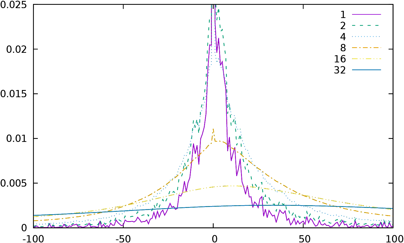
| Figure 10: Example of a distribution of Rw−b from a
Fischer-Spassky game, for 1, 2, 4, 8, 16
and 32 pairs of moves. The x-axis scale is in centipawns. |
Then Rn is a normal
distribution of parameters µn=nµ and
σn=√nσ: the distribution “shifts” to the right
if µ is positive (p1 is the strongest player), and to the left
if µ is negative (p2 is the strongest player), and it
also “flattens”, i.e., it is much less centered around
µn. If we consider that a victory is having a
score S>b after n moves, then its probability is
∫b+∞ Rn =
(1−erf(b−nµ/√2nσ))/2.
Respectively, a draw
would be
∫−b+b Rn =
(erf(b−nµ/√2nσ)+
erf(b+nµ/√2nσ))/2
and a defeat
∫−∞−b Rn =
(1−erf(b+nµ/√2nσ))/2.
If we compute the limit when n→
+∞ we see that all the density of the distribution goes to
either side depending on the sign of µ: if player p1 is the
strongest (respectively weakest) µ is positive (respectively negative)
and, at infinity, all games end in wins (respectively defeats) for
White. Intuitively, the fundamental flaw in the hypothesis is that a
chess game is finite and thus ends after the score reaches some
given limit on either side, something we are not taking into account
here, thus taking simply the limit is not correct either.
Instead of
fitting the model to the data
by using parameters k1, k2 and the elements of the gain vector,
it is possible to compute the correlation of the estimated gain
(here31
0.5∫−b+b Rn0 + 1 ∫b+∞ Rn0) with
the actual result of the game as a function of n0 and b. The
results are displayed in
Figure 11, for n0=0,⋯,95 and
b=0.0,0.2,⋯7.6,7.8.
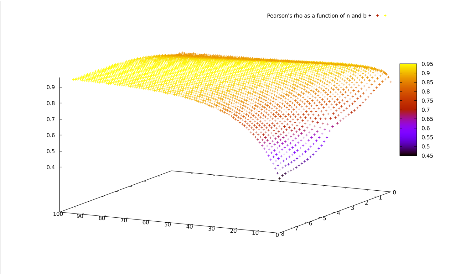
| Figure 11: ρ as a function of n0 (from 0 to 95) and b (from
0 to 8) |
They are excellent, with a maximal value for ρ of 95%, much
higher than any other value we ever had.
There are many tuples
(n0,b) for which the correlation is around 95%.
| Figure 12:
Value of the optimal b (left), and of ρ with the optimal
b (right), as a function of n0
|
In the left part of Figure 12 we display the optimal value of
b as a function of n0. As predicted by the normal
distribution approximation, b grows almost linearly with n0. The
correlation is rising fast and 94% is reached for n0=29 and b=2.2.
4.3.2 Whole career
The gain covariance representation is only able to provide results for
head to head confrontations. It is not a scalar value and thus cannot
be plot like the aggregated conformance indicator. However,
as all results are available for all World Champions
for all their active years, it is now possible to predict the outcome
of a match between any World Champion from any active year with any other Champion
taken in any active year; it is even possible to predict
the result of Fischer 1970 against Fischer 1971.
A first experiment was done using the most basic
settings, i.e., setting n0 to 0 (which is exactly Ferreira’s
interpretation).
This “Battle Royale” which consisted in predicting the result of
around 300,000 possible match combinations, was performed in a few
minutes by the computer. The result is a 14 megabytes database which gives
the predicted outcome of the games between any two World Champions for
any year.
Now, for each player, the “best year” was found by
searching for the year where the player had the largest number of victories
against all other players and all other years. The results were as
follows:
Alekhine (1921),
Anand (2010),
Botvinnik (1945),
Capablanca (1918),
Carlsen (2013),
Euwe (1934),
Fischer (1972),
Karpov (1988),
Kasimdzhanov (2013),
Kasparov (2000),
Khalifman (2013),
Kramnik (2007),
Lasker (1907),
Petrosian (1962),
Ponomariov (2013),
Smyslov (1964),
Spassky (1965),
Steinitz (1872),
Tal (1981),
Topalov (2006).
Some results might seem surprising. For example, it is usually
supposed that Botvinnik
had been playing at his peak when he was World Champion (from
1948 to 1963). However, when looking carefully, 1945 was an exceptional year for
him: he won the USSR Championship with an amazing 15 out of 17
possible points, at a time when there were almost no international
competitions, and where the USSR Championship was probably the
strongest possible competition. So it is quite possible that 1945 is indeed the year he
played at his best. A second quite surprising results is Tal’s
best years. But there again Tal reached his peak ELO rating in 1980,
far from the years he was World Champion.
Then we extracted from the database the results of the head to head
predictions for these players taken this particular year.
The results are displayed in Table 7. The results are not
exactly symmetric as playing as White and playing as Black give
different results as explained above.
|
| Ca | An | Kr | Ka | To | Fi | Kh | Po | Bo | Ka | Ka | Ca | La | Pe | Ta | Sm | Eu | Al | Sp | St |
|
Carlsen | | 50 | 50 | 51 | 51 | 52 | 52 | 52 | 52 | 53 | 53 | 53 | 53 | 54 | 54 | 54 | 54 | 54 | 54 | 55 |
|
Anand | 50 | | 50 | 50 | 51 | 51 | 51 | 52 | 52 | 52 | 52 | 53 | 53 | 53 | 53 | 53 | 53 | 54 | 54 | 55 |
|
Kramnik | 50 | 50 | | 50 | 51 | 51 | 51 | 52 | 52 | 52 | 52 | 53 | 53 | 53 | 53 | 53 | 53 | 53 | 54 | 55 |
|
Kasparov | 49 | 50 | 50 | | 50 | 51 | 51 | 51 | 52 | 52 | 52 | 52 | 53 | 53 | 53 | 53 | 53 | 53 | 53 | 55 |
|
Topalov | 49 | 49 | 49 | 50 | | 50 | 51 | 51 | 51 | 51 | 52 | 52 | 52 | 52 | 52 | 53 | 53 | 53 | 53 | 54 |
|
Fischer | 48 | 49 | 49 | 49 | 50 | | 50 | 50 | 51 | 51 | 51 | 51 | 52 | 52 | 52 | 52 | 52 | 52 | 53 | 54 |
|
Khalifman | 48 | 49 | 49 | 49 | 49 | 50 | | 50 | 51 | 51 | 51 | 51 | 52 | 52 | 52 | 52 | 52 | 52 | 53 | 54 |
|
Ponomariov | 48 | 48 | 48 | 49 | 49 | 50 | 50 | | 50 | 50 | 51 | 51 | 51 | 51 | 51 | 52 | 52 | 52 | 52 | 53 |
|
Botvinnik | 48 | 48 | 48 | 48 | 49 | 49 | 49 | 50 | | 50 | 50 | 51 | 51 | 51 | 51 | 51 | 51 | 52 | 52 | 53 |
|
Kasimdzhanov | 47 | 48 | 48 | 48 | 49 | 49 | 49 | 50 | 50 | | 50 | 51 | 51 | 51 | 51 | 51 | 51 | 51 | 52 | 53 |
|
Karpov | 47 | 48 | 48 | 48 | 48 | 49 | 49 | 49 | 50 | 50 | | 50 | 51 | 51 | 51 | 51 | 51 | 51 | 52 | 53 |
|
Capablanca | 47 | 47 | 47 | 48 | 48 | 49 | 49 | 49 | 49 | 49 | 50 | | 50 | 50 | 51 | 51 | 51 | 51 | 51 | 53 |
|
Lasker | 47 | 47 | 47 | 47 | 48 | 48 | 48 | 49 | 49 | 49 | 49 | 50 | | 50 | 50 | 50 | 50 | 51 | 51 | 52 |
|
Petrosian | 46 | 47 | 47 | 47 | 48 | 48 | 48 | 49 | 49 | 49 | 49 | 50 | 50 | | 50 | 50 | 50 | 51 | 51 | 52 |
|
Tal | 46 | 47 | 47 | 47 | 48 | 48 | 48 | 49 | 49 | 49 | 49 | 49 | 50 | 50 | | 50 | 50 | 50 | 51 | 52 |
|
Smyslov | 46 | 47 | 47 | 47 | 47 | 48 | 48 | 48 | 49 | 49 | 49 | 49 | 50 | 50 | 50 | | 50 | 50 | 51 | 52 |
|
Euwe | 46 | 47 | 47 | 47 | 47 | 48 | 48 | 48 | 49 | 49 | 49 | 49 | 50 | 50 | 50 | 50 | | 50 | 51 | 52 |
|
Alekhine | 46 | 46 | 47 | 47 | 47 | 48 | 48 | 48 | 48 | 49 | 49 | 49 | 49 | 49 | 50 | 50 | 50 | | 50 | 52 |
|
Spassky | 46 | 46 | 46 | 47 | 47 | 47 | 47 | 48 | 48 | 48 | 48 | 49 | 49 | 49 | 49 | 49 | 49 | 50 | | 51 |
|
Steinitz | 45 | 45 | 45 | 45 | 46 | 46 | 46 | 47 | 47 | 47 | 47 | 47 | 48 | 48 | 48 | 48 | 48 | 48 | 49 | |
| Table 7: Head to head match result predictions between different
World Champions in their best year using the Covariance
indicator with n0=0 |
A second similar experiment was done, with different
parameters. Here n0=32 and b=2.4, which is supposed to yield
“better” results. These results are somewhat
different from the previous ones. The best years are:
Alekhine (1931),
Anand (2011),
Botvinnik (1945),
Capablanca (1924),
Carlsen (2013),
Euwe (1934),
Fischer (1971),
Karpov (1977),
Kasimdzhanov (2013),
Kasparov (2001),
Khalifman (2013),
Kramnik (2000),
Lasker (1907),
Petrosian (1962),
Ponomariov (2013),
Smyslov (1964),
Spassky (1970),
Steinitz (1873),
Tal (1967),
Topalov (2005).
The results are presented in Table 8. We see that
Fischer fell to almost the end of the ranking, while Capablanca almost
reached the top.
|
| Ka | Kr | Ca | Ca | Ka | An | Pe | Kh | Ka | Sm | La | Bo | Eu | To | Ta | Po | Al | Sp | Fi | St |
|
Kasparov | | 51 | 51 | 52 | 52 | 53 | 53 | 53 | 53 | 54 | 55 | 55 | 57 | 58 | 60 | 60 | 61 | 64 | 66 | 69 |
|
Kramnik | 49 | | 50 | 51 | 51 | 52 | 52 | 53 | 53 | 53 | 54 | 54 | 57 | 57 | 59 | 60 | 60 | 64 | 65 | 68 |
|
Carlsen | 49 | 50 | | 51 | 51 | 52 | 52 | 53 | 53 | 53 | 54 | 54 | 57 | 57 | 60 | 60 | 60 | 64 | 65 | 69 |
|
Capablanca | 48 | 49 | 49 | | 50 | 51 | 51 | 51 | 52 | 52 | 53 | 53 | 55 | 56 | 58 | 58 | 58 | 62 | 63 | 66 |
|
Karpov | 48 | 49 | 49 | 50 | | 51 | 51 | 51 | 51 | 52 | 52 | 53 | 55 | 55 | 58 | 58 | 58 | 62 | 63 | 66 |
|
Anand | 47 | 48 | 48 | 49 | 49 | | 50 | 51 | 51 | 51 | 52 | 52 | 55 | 55 | 58 | 58 | 58 | 62 | 63 | 66 |
|
Petrosian | 47 | 48 | 48 | 49 | 49 | 50 | | 50 | 51 | 51 | 52 | 52 | 54 | 55 | 57 | 57 | 58 | 61 | 63 | 65 |
|
Khalifman | 47 | 47 | 48 | 49 | 49 | 50 | 50 | | 50 | 51 | 51 | 52 | 54 | 54 | 57 | 57 | 57 | 61 | 62 | 65 |
|
Kasimdzhanov | 47 | 48 | 48 | 49 | 49 | 50 | 50 | 50 | | 51 | 51 | 52 | 54 | 54 | 57 | 57 | 57 | 61 | 62 | 65 |
|
Smyslov | 46 | 47 | 47 | 48 | 48 | 49 | 49 | 49 | 49 | | 50 | 51 | 53 | 53 | 56 | 56 | 56 | 60 | 61 | 64 |
|
Lasker | 46 | 46 | 46 | 48 | 48 | 48 | 48 | 49 | 49 | 50 | | 50 | 53 | 53 | 55 | 56 | 56 | 60 | 61 | 63 |
|
Botvinnik | 45 | 46 | 46 | 47 | 47 | 48 | 48 | 48 | 49 | 49 | 50 | | 52 | 53 | 55 | 55 | 56 | 59 | 61 | 63 |
|
Euwe | 43 | 44 | 43 | 45 | 45 | 45 | 46 | 46 | 46 | 47 | 47 | 48 | | 50 | 53 | 53 | 53 | 57 | 58 | 61 |
|
Topalov | 42 | 43 | 43 | 45 | 45 | 45 | 45 | 46 | 46 | 47 | 47 | 47 | 50 | | 52 | 53 | 53 | 57 | 58 | 61 |
|
Tal | 40 | 41 | 40 | 42 | 43 | 43 | 43 | 43 | 44 | 45 | 45 | 45 | 47 | 48 | | 50 | 51 | 55 | 55 | 58 |
|
Ponomariov | 40 | 41 | 40 | 42 | 42 | 43 | 43 | 43 | 43 | 44 | 45 | 45 | 47 | 48 | 50 | | 51 | 54 | 55 | 59 |
|
Alekhine | 40 | 40 | 40 | 42 | 42 | 42 | 43 | 43 | 43 | 44 | 44 | 44 | 47 | 47 | 49 | 50 | | 54 | 55 | 58 |
|
Spassky | 36 | 36 | 36 | 38 | 38 | 38 | 39 | 39 | 39 | 40 | 40 | 41 | 43 | 43 | 46 | 46 | 46 | | 51 | 54 |
|
Fischer | 34 | 35 | 35 | 37 | 37 | 37 | 38 | 38 | 38 | 39 | 39 | 40 | 42 | 42 | 45 | 45 | 45 | 49 | | 53 |
|
Steinitz | 31 | 32 | 31 | 34 | 34 | 34 | 35 | 35 | 35 | 36 | 37 | 37 | 39 | 39 | 42 | 42 | 43 | 46 | 47 | |
| Table 8: Head to head match result predictions between different
World Champions in their best year using the Covariance
indicator with n0=32 and b=2.4 |
There are some common factors in both rankings:
according to the conformance indicator,
the level of
chess has been increasing through the years.
There are more “contemporary” players
in the top of this ranking than players from the previous generations.
There are also important differences; this is probably telling us that
this indicator is somewhat “flawed” for the same reasons as the aggregated
conformance indicator: it does not take into account the “context”
of the move: making a small mistake when the game is already lost or
won has not the same significance as making it when the game issue is
not decided yet, while this indicator is “averaging” them. A longer
study is necessary to assess exactly why some players are more
“unstable” than others. However the example of Fischer is somewhat
significant: let us remember that, with the aggregated conformance
indicator, Fischer was also “topping” the rankings regarding his
ability to find the exact “best” move, but was much more “ordinary”
when considering aggregated conformance for δ ≤ 0.3. This
might mean that he was playing perfectly very often but could also
make “larger” mistakes more often than some other players. The
question again is: under what circumstances was he making such mistakes?
This problem is
exactly what I expect to correct with the Markovian predictor.
4.3.3 Predicting the results of World Championships
Below, we compare the score predicted for World Championships by
the Covariance predictor to (1) the actual score and to (2) the score predicted
using ELO tables as we did for the accumulated conformance
indicator in subsection 4.2.4. The results are also presented
in Table 5 in column Covs. The predictor is computed
using n0=32 and b=2.4.
The mean
difference between the actual score and the accumulated conformance
predicted score is 8% on all championships and of 9% on the 11 World
Championships for which the ELO predictor is available. So, in a quite
paradoxical way, the covariance predictor is less efficient than the
accumulated conformance predictor, even if it is better correlated to
the result of individual games.
4.4 The Markovian predictor
The Markovian predictor presented in section 3.4
relies on transition matrices which represent for each value of the
evaluation function the probability of the value of the evaluation
function in the next step. This solves the problem presented
in the previous sections regarding the “context” of a
mistake. However, to operate properly, the Markovian predictor requires
a large amount of data to build matrices which are statistically
significant. Thus it is not possible to use it and/or validate it on a
single game, because there are simply not sufficient data. The Markovian
predictor is designed to evaluate a player on a collection of games
and not on single games, which is quite different from the previous
two. In the next three subsections we explain first how to compute
efficiently transition matrices (4.4.1), then we compute the
Markovian predictor on whole careers (4.4.2) and finally we
use it to compute predictions for World Championships matches
(4.4.3).
4.4.1 Computing efficiently transition matrices
There are two antagonist objectives when building transition
matrices. On the one hand, the more classes (rows) we have, and the better
is the modeling of the stochastic process. On the other hand,
it is important to have “sufficient” moves
played in each class (row of the matrix), in order to have a significant
statistical estimation of all the parameters of this class.
As matrices are computed for each year the player was active, it is
mandatory
to set a lower bound to the number of moves played during one year to
declare the player “active”. This is not as simple as it seems. Some
players (such as Botvinnik for example) used to play a low number of
games between championships. Some retired for long periods (Fischer
retired for 18 months from mid 68 to mid 70). After examining
the careers of different players, the lower bound for the number of
moves played was set to 500, which seems to make a proper distinction
between years of activity and years of semi-retirement (Fischer played
some demonstration games in 1969 that cannot be considered as
significant).
The second parameter to choose is the value of the upper and lower
bounds binf and bsup. There again, the larger the value, the
better the prediction of the process should be. However, here
again, it is important to have sufficient positions when the
evaluation of the current game is below binf and above
bsup. A statistical analysis of the games of the players
considered shows that it is difficult to find many moves played below
binf if binf is too large. There are two main reasons: on
the one hand, world class
players usually do not lose their games; on the other hand, when they
are in this kind of situation, they seem to resign pretty soon, which
reduces the number of moves available. The same goes on a lesser
extent for bsup; even if their opponents are less strong, they
usually resign pretty fast when the position becomes bad against a
world class player. The side effect of choosing bsup too low
(respectively binf too high), is that the expected percentage of won
(respectively lost) games will be higher, while the expected percentage of
drawn games will be lower.
The underlying interpretation of the stationary vector
is that the last
component of the stationary vector represents games won and that the
expected gain should be 1 for this class32, that
the “middle” elements correspond to draw with unbalanced material,
while the first component represent games lost. We are thus using
e=(0,0.5⋯,0.5,1) as the gain vector, and we compute the
expected output of the game by making the scalar product of the
stationary vector π with the gain vector e.
Let us notice first that we cannot use, to compute the
values of the e vector, the same optimization method as in
the previous section for the covariance gain vector.
The optimization in the previous section can be performed
because we can compute for each game the expected result,
compare it to the actual result and perform a least squares
method to reduce the discrepancy. The Markovian method works only
on a large set of games, because it requires a large amount of
data. It is impossible to compute one matrix for one game. We
could have performed an optimization by computing the matrix on a
large number of games, and then compare the expected average
computed outcome with the actual one. However, we decided not to
perform this optimization step, for different reasons.
-
On the one hand, the
Markovian process and the computation of the stationary vector takes
into account the idea that a high value (low value) leads usually
the game to a
higher value (respectively lower value) and ultimately to one of the
extremal class. Thus the probabilities represented in the stationary
vector by the “not extremal” classes are really the probabilities of
not going
to one of the extremal class when t→ +∞, and thus
they represent a draw with more or less unbalanced
material.
- On the other hand, the gain expectancy associated to a
class cannot be estimated
in an intrinsic way: it depends, not only on the player, but also on
his opponents, as we can only estimate it from the player’s
games. Moreover, in a game between two players, what vector do we
choose: player one’s vector, player two’s vector or an average of
the two? To solve this
last problem we could try to find
a general “gain expectancy” vector, either by trying to make a
least square regression on actual data, or by deducing it
from many games played by the computer in
autoplay. But using this interpretation would defeat the very idea that
different human
players have different capacities, and should thus have different
“gain vectors” if we choose to interpret them that way.
- Last, but not least, not performing any “fitting” of the
model to the data guarantees that the Markovian model remains, in a
way, “pure”, as it is completely
independent of the players on which the study is performed. The only
thing that depends on the player is its Markovian matrix.
This choice will be discussed
in subsection 4.4.3, when I will compare the “pure” Markovian
model to the other predictors regarding its capacity to predict the outcome of a set
of games.
It is possible to try to have an idea of the estimation
of the induced error.
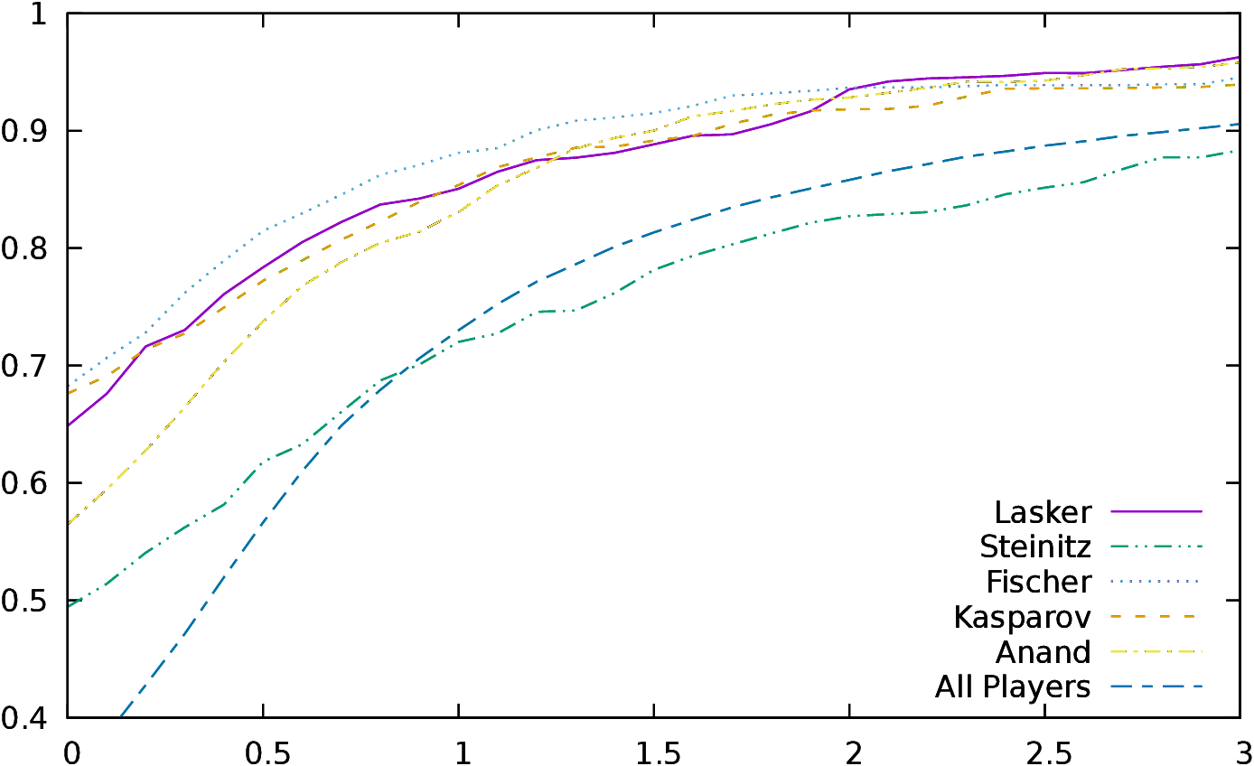
| Figure 13: Expected value of gain as a function of the highest
evaluation reached in the game |
In Figure 13, we see for some selected players the expected
value of
the result as a function of the evaluation of the best position
reached by the player during the game (the statistics are computed on
all games). For example, if we consider
Emmanuel Lasker, he won on the average 0.65 points when,
during a game, he reached at least once a position valued 0. He won 0.85
points when he reached at least once a position valued 1.00 (100cp), 0.94
points for 2.00, 0.96 points for 3.0033. So we make an approximation
of 0.06 points when setting bsup to 2.00, and an error of 0.04
points when setting it to 3.00.
These values are approximately the
same for all the World Champions considered in this study, except for
Wilhelm Steinitz,
who is clearly below. We also notice that they are
well over the “All Players” curve34.
The difference between 2.0 and 3.0 is
small and thus a reasonable choice seems to be +2 as
bsup. The same study with quite identical results can be done for binf.
+2/-2 is also the value chosen as the limit of won/lost
games by Guid and Bratko in their study, and these values give us sufficient
moves in the extremal classes to have statistical consistent
samples.
The last value to choose is the grain g, which is the size of each class,
and which thus sets also the number of classes (rows and columns of the
matrices).
The statistical analysis of position evaluations showed
that choosing a
single g was a poor idea. Moves made are usually made when the
evaluation is close to 0, and their distribution is “Gaussian”.
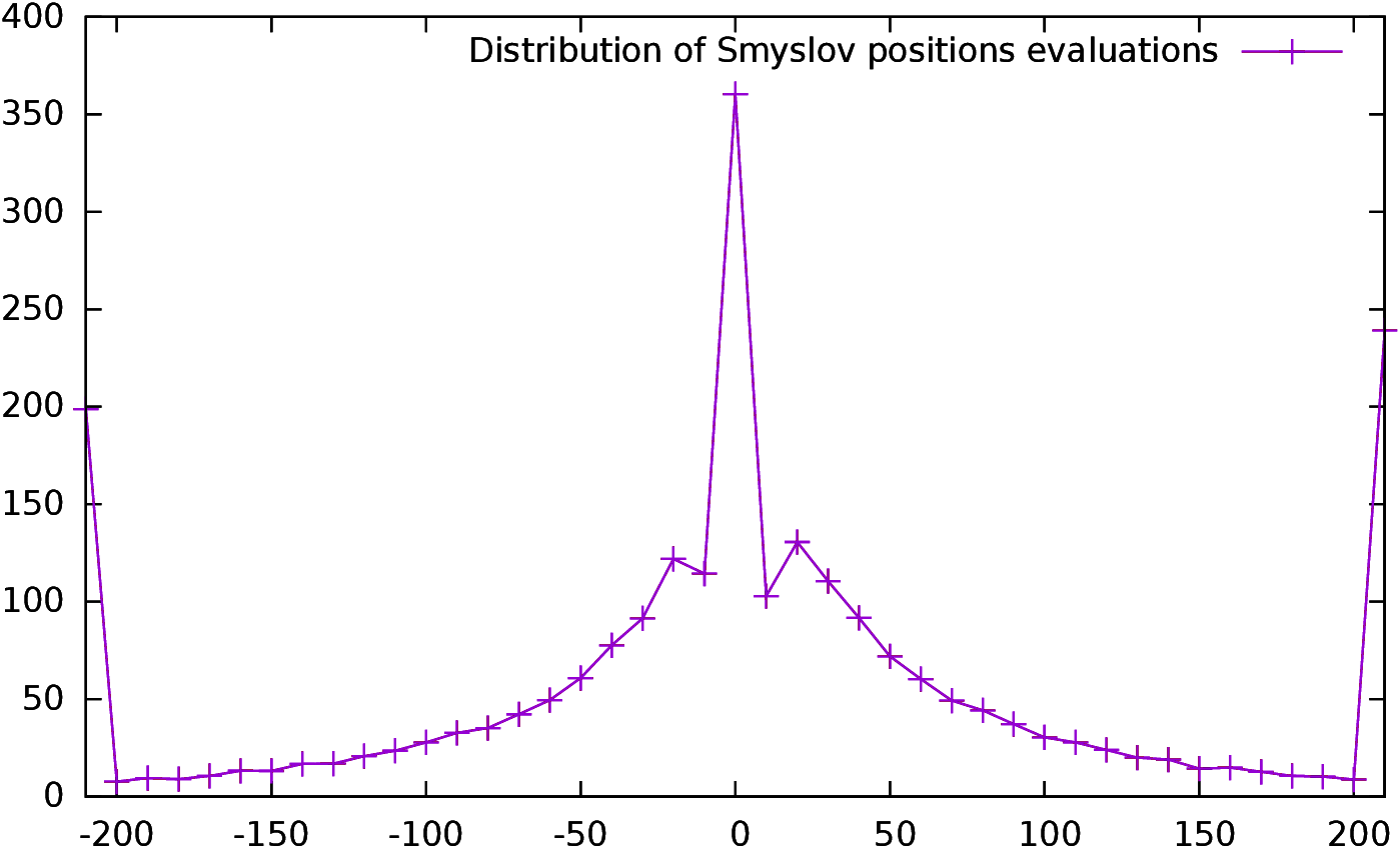
| Figure 14: Average number of positions by year as a function of the
evaluation of the positions |
Figure 14 represents the distribution of the
evaluation of the positions of Vassily Smyslov during his extremely
long and competitive career. binf and bsup were set to
-2/+2, and g was set to 10 centipawns. -210 represents all
positions with an evaluation of -200 or below, -200 the positions with
an evaluation between -200 and -190 and so on.
There are
151,489 positions over 60 years,
or an average of almost 2500 positions by year (5 times the limit of
500 moves).
The positions evaluated as 0 are a class of their own as it is the
positions which are
draws, and there are lots of them. This is understandable
as players often keep on playing in some positions that computer programs,
especially with endgame databases, identify early as draws. Some
classes are ridiculously small; for example the 200 class contains
only 8 positions/year, and this is only on the average. A full
statistical analysis for all players and all
years demonstrated that with this distribution, there were some
classes which were empty during “active” years.
Thus the number of classes was reduced to 19,
and the width of each class was computed in order to better balance the
number of elements by class. As the distribution looked Gaussian, the
size of classes were set to follow a logarithmic function. The three
special classes (above bsup, below binf and 0) are kept
unchanged, while a scaling factor is applied to the size of classes
equal to:
|
f= | | e−v/100−e−bsup/100 |
|
| e0−e−bsup/100 |
|
for v>0
|
A similar symmetric factor was applied for v<0. The results are
presented in Figure 15.
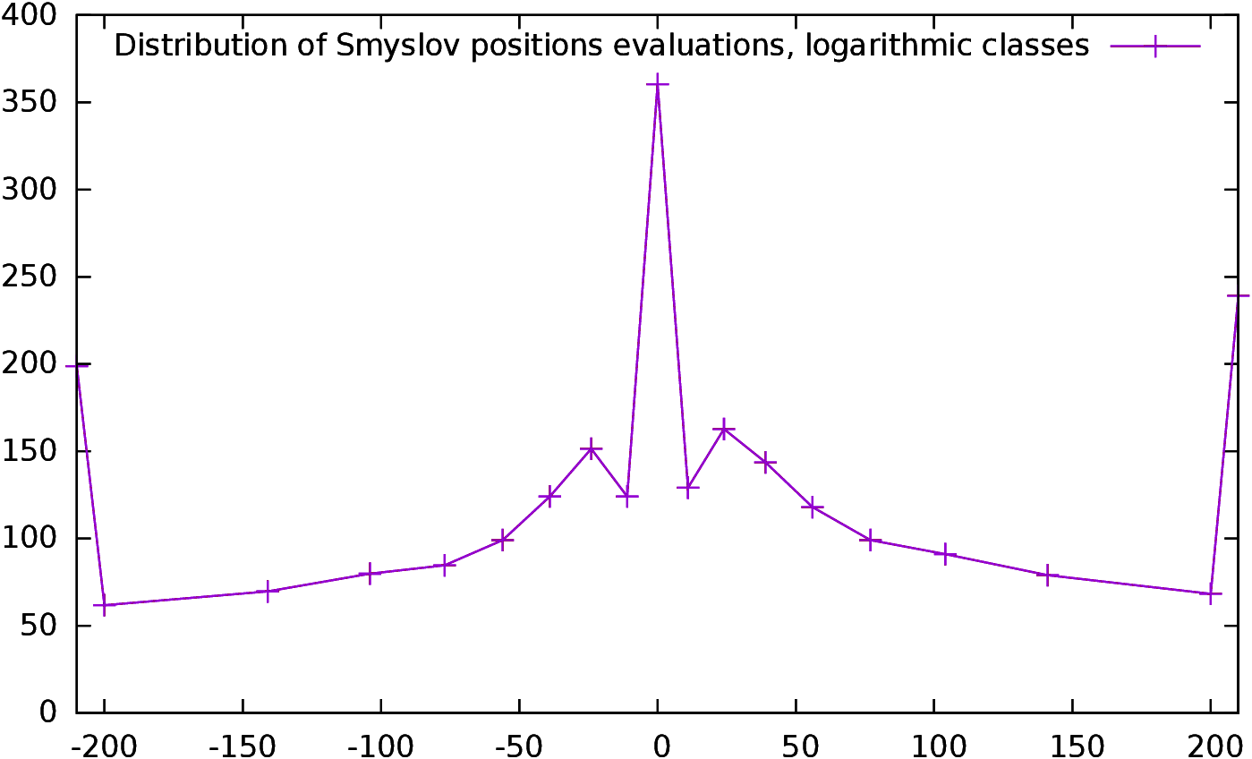
| Figure 15: Average number of positions by year as a function of the
evaluation of the positions, using logarithmic size
classes |
The central class (positions
evaluated to 0) and the classes representing positions over bsup
or below binf are classes of their own. The classes closest to zero
on either side are 10cp wide, and the width of classes grows as we get
further from 0, with the last classes being 50cp wide.
This new distribution gives classes with a minimal number of
around 50 elements, which is a significant sample.
A last improvement was made to the system. In order to stabilize the
matrices, and to prevent jumps from year to year, the positions of the
previous years are taken into account, but with an exponential
forgetting factor of 2 (positions of the previous year count as half,
position of n−2 count as one quarter, etc.).
It would have probably been better to use a sliding time window, but
unfortunately dates in the database are often reduced to the year and
do not mention the month.
It is now possible to compute the transition matrices, which are
square 19x19 matrices. Taking again as an example Fischer and Spassky
in 1971, the new stationary vector is now:
|
v | = | (0.10,0.02,0.01,0.01,0.02,0.02,0.02,0.02,0.02 |
| | | 0.11,0.03,0.03,0.04,0.04,0.04,0.03,0.02,0.07,0.36)
|
|
This represents a 36% win for Fischer and a 10% win for
Spassky35.
A last important comment: as with any statistical methods, data are
aggregated here solely based
on some specific criteria (the value of the evaluation function),
disregarding all other
parameters. For example, the material still present on the
board is not taken into account, while it seems pretty clear that the
variations in the evaluation function are not of the same nature at
the beginning of a game and at the end of a game.
It would be interesting to try to create more complex classes, using
the material present on the board as a second criteria. This is
probably difficult to do; even if only three main
subclasses are used (opening, mid-game and ending), this would
subdivide each
class into three classes, and the problem of having sufficient
samples would arise again.
4.4.2 Whole career
As in subsection 4.3.2, a “Battle Royale” was performed,
and for each player, the “best year”
was found by
searching for the year where the player had the largest number of victories
against all other players and all other years. The results were as
follows:
Carlsen: 2013,
Kramnik: 1999,
Fischer: 1971,
Kasparov: 2001,
Anand: 2008,
Khalifman: 2010,
Smyslov: 1983,
Petrosian: 1962,
Karpov: 1988,
Kasimdzhanov: 2011,
Botvinnik: 1945,
Ponomariov: 2011,
Lasker: 1907,
Spassky: 1970,
Topalov: 2008,
Capablanca: 1928,
Euwe: 1941,
Tal: 1981,
Alekhine: 1922,
Steinitz: 1894.
|
| Ca | Kr | Fi | Ka | An | Kh | Sm | Pe | Kp | Ks | Bo | Po | La | Sp | To | Ca | Ta | Eu | Al | St |
|
Carlsen | | 52 | 54 | 54 | 57 | 58 | 57 | 58 | 56 | 60 | 61 | 59 | 60 | 61 | 61 | 64 | 66 | 69 | 70 | 82 |
|
Kramnik | 49 | | 52 | 52 | 55 | 56 | 56 | 57 | 55 | 59 | 60 | 58 | 60 | 60 | 60 | 63 | 65 | 68 | 70 | 83 |
|
Fischer | 47 | 49 | | 51 | 53 | 57 | 56 | 57 | 56 | 59 | 60 | 60 | 61 | 61 | 62 | 64 | 68 | 70 | 73 | 85 |
|
Kasparov | 47 | 49 | 50 | | 53 | 54 | 54 | 54 | 53 | 57 | 58 | 56 | 56 | 58 | 58 | 60 | 62 | 66 | 68 | 82 |
|
Anand | 44 | 46 | 48 | 48 | | 54 | 52 | 53 | 53 | 57 | 56 | 57 | 57 | 59 | 59 | 62 | 64 | 69 | 71 | 86 |
|
Khalifman | 43 | 45 | 44 | 47 | 47 | | 50 | 51 | 52 | 53 | 54 | 55 | 55 | 56 | 56 | 60 | 62 | 64 | 67 | 79 |
|
Smyslov | 43 | 45 | 45 | 47 | 49 | 51 | | 50 | 51 | 53 | 55 | 54 | 54 | 54 | 55 | 59 | 63 | 64 | 68 | 82 |
|
Petrosian | 43 | 44 | 45 | 47 | 49 | 50 | 51 | | 52 | 53 | 54 | 54 | 55 | 55 | 56 | 59 | 63 | 63 | 67 | 80 |
|
Karpov | 44 | 46 | 45 | 48 | 48 | 49 | 50 | 49 | | 51 | 52 | 52 | 52 | 52 | 52 | 56 | 58 | 60 | 63 | 76 |
|
Kasimdzhanov | 41 | 43 | 42 | 45 | 45 | 48 | 48 | 48 | 50 | | 52 | 52 | 52 | 54 | 53 | 56 | 60 | 62 | 65 | 80 |
|
Botvinnik | 40 | 41 | 41 | 44 | 45 | 48 | 46 | 48 | 49 | 49 | | 50 | 54 | 52 | 52 | 56 | 60 | 60 | 64 | 80 |
|
Ponomariov | 42 | 43 | 41 | 45 | 44 | 47 | 47 | 47 | 49 | 49 | 51 | | 51 | 52 | 52 | 55 | 58 | 59 | 62 | 77 |
|
Lasker | 41 | 41 | 40 | 45 | 44 | 46 | 47 | 46 | 49 | 49 | 48 | 50 | | 51 | 50 | 54 | 58 | 59 | 63 | 78 |
|
Spassky | 40 | 41 | 40 | 43 | 42 | 45 | 47 | 46 | 48 | 47 | 49 | 49 | 50 | | 51 | 53 | 58 | 57 | 61 | 75 |
|
Topalov | 40 | 41 | 39 | 44 | 42 | 45 | 46 | 45 | 49 | 48 | 49 | 49 | 50 | 51 | | 54 | 57 | 57 | 61 | 75 |
|
Capablanca | 37 | 38 | 37 | 41 | 39 | 42 | 42 | 42 | 45 | 45 | 45 | 47 | 47 | 48 | 47 | | 53 | 54 | 59 | 76 |
|
Tal | 35 | 36 | 34 | 39 | 37 | 39 | 39 | 38 | 43 | 41 | 41 | 43 | 43 | 43 | 44 | 48 | | 49 | 54 | 72 |
|
Euwe | 32 | 33 | 32 | 36 | 32 | 37 | 37 | 38 | 41 | 39 | 41 | 42 | 43 | 44 | 44 | 47 | 52 | | 56 | 75 |
|
Alekhine | 31 | 31 | 29 | 34 | 30 | 35 | 33 | 35 | 38 | 36 | 37 | 39 | 38 | 40 | 40 | 43 | 47 | 45 | | 69 |
|
Steinitz | 20 | 19 | 17 | 20 | 16 | 22 | 19 | 22 | 25 | 22 | 22 | 25 | 24 | 27 | 27 | 26 | 30 | 27 | 33 | |
| Table 9: Head to head match result predictions between different
World Champions in their best year |
The results are displayed in Table 9. Here again, the results are not
exactly symmetric as playing as White and playing as Black give
different results as explained above.
It is not straightforward to deduce an absolute
ranking from it; for example, Tal is performing consistently better than Euwe
against stronger players, but is losing to Euwe (with a small margin).
According to this predictor too, it is clear that the level of
chess has been increasing through the years. A group of 4
players (Carlsen, Kramnik, Fischer, Kasparov) is ahead of
the pack, while a group of 3 (Euwe, Alekhine and
Steinitz) is trailing below (Steinitz being way below the others).
The in-between players are close to each other.
The results are not exactly the same as those found with the
covariance indicator (Fischer for example has a better ranking here),
however they are very close.
4.4.3 Predicting the results of World Championship using the Markovian model
Below, we compare the score predicted for World Championships by
the Markovian predictor to the actual score and to the score predicted
using ELO tables as we did for the accumulated conformance
indicator in subsection 4.2.4 and for the covariance
predictor in subsection 4.3.3. The results are also presented
in Table 5 in column Ms.
The difference between the actual score and the
Markovian predicted score is 3.6% on all Championships and of 4.4% on the 11 World
Championships for which the ELO predictor is available. The Markovian
predictor is thus the best of the three, even if
the sample of available data is too small to have a definitive conclusion.
It would have been interesting to do a more thorough comparison of the
three predictors, but this
was out of reach of this study, as much more computing power is required.
5 Conclusion
Statistical studies give correlation information, they do not directly
provide causality, and interpreting them requires some perspective.
The cumulative conformance indicator presented in this article measures the
capacity to play “like” a very strong computer program, even if its
interpretation, as discussed in subsection 4.2.1, is a little
bit more complex.
Believing
that this indicator is a measure of the real “strength” of a player is
plausible, as I have demonstrated along this
article that conformance was highly correlated with the game
outcome, and we know that computer programs are currently much
stronger than human beings. However, it is important to remember that
the indicator has been built and verified only on world class players,
and extending it to lesser players would require more
experimentation. Moreover, we have seen that this indicator has some
drawbacks, as it requires a delicate fitting to the data, and does not
take into account the context of the moves played.
The distribution vector is in a sense “richer” than the scalar
cumulative conformance indicator. However, it requires also to be
fitted to the data, and its results regarding its ability to predict
the results of matches seem less good than the other two.
The Markovian predictor gives very interesting
prediction results which are better on this limited sample than the
two other predictors and even better than the usual ELO
predictor. It is the “purest” of the three, as it does not require
any specific fitting, and the Markovian interpretation is apparently
the “soundest” of the three. As it is an intrinsic predictor which does not depend on
the evaluation of other players, it could be a possible replacement of
the usual ELO predictor, even if a clear drawback is the fact that it
is a composite predictor, which enables only to compare two players,
but not to build simply a total order between players. However, it
could be possible to build a ranking by simulating all possible
confrontations between players of the same class, and averaging the
results.
There remains a plethora of things to do. Below we mention seven of them.
-
It is necessary to evaluate much
more games, and this is definitely possible. A rough estimation done
with Chessbase shows that there
are certainly less than 500,000 regular time games which would have to
be evaluated in
order to assess all games where both players are above 2500
ELO. This is 25 times the number of games assessed in this
study, but it is definitely within our grasp. On a Xeon E5-2680 v2 @ 2.80GHz
processor, this would require around 500,000 hours of CPU time to have
the quality of evaluation of this study which used old HE 6262 AMD
processors. 500,000 hours is not much regarding the capacity of HPC
centers: it would represent 40 hours for the CALMIP EOS computer,
which was ranked 183 in the TOP 500 list as of 06/2014, and only 10
minutes on the Tianhe-2 (the speedup is completely linear with the
number of cores as the problem is fully parallel).
Even
evaluating the complete Chessbase database after removing games with
fast time controls is now possible.
- The database must be checked again.
Properly filtering the database is a difficult problem. Finding time
controls is usually difficult, and it is
sometimes necessary to guess them from the name of the
tournament. Also, cleaning up the history of the games to suppress move
repetitions would probably be beneficial.
Moreover there are little glitches (such as players who have exactly
the same names, while they are not the same player) which should be
solved before going further. Cooperating with people developing
chess databases would definitely be a clear advantage.
- Results should be compared by using different chess engines to
evaluate moves, to see what results are “engine dependent” or
“engine independent”. It is almost certain that some of them
depend on the program used, as the evaluation function is different
from program to program. However, what is probably more important is
the similarity in the ranking of moves. Further experiments are
required, even if there has already been such
studies [GB11], which mainly conclude that the ranking
between chess programs is usually consistent.
- More data should be gathered. It would have been beneficial to store more information
during the search. This would have enabled to compute other indicators
(such as Sullivan’s complexity) and test other approaches, such as
Haworth and Regan’s.
- The conformance indicator, gain distribution vector or Markovian
matrices should probably be computed
separately for White and for Black, as players seem to play
differently when they are playing as Black or as White.
This is an aside, but interesting result, of this study.
- Some of the problems found in this study might be a consequence
of the structure of the evaluation functions in chess, which cannot
be mapped easily to the probability of winning a game. So, on the
one hand, a parallel
statistical work regarding evaluation functions could be
performed in order to better understand this mapping. On the other
hand, applying this methodology to a game such as Othello/Reversi
with an engine using an evaluation function returning the probability of
winning would also provide useful information.
- Results might depend on the fact that the model has
been fitted36 to a particular type of players,
namely world class
players, and even more generally to human beings. The psychological
biases that appear when playing as Black, or when playing a little
recklessly in inferior positions would not appear in games between
computers. So it would be extremely interesting to gather games
played by computers at blitz level, and to see how the results are
modified.
However, the intermediate results show that the level in
chess has raised through the years, and that the young players of our
days are extremely strong. This is probably to be expected: Magnus
Carlsen was born in 1990, which means that he had at his disposal
for training during almost all his life a small computing device at
home which was stronger than any existing player ever, and databases
containing all the games ever played. The drawback is
probably that the current chess games are sometimes considered as
“dull” by some commentators: there are very few mistakes made, and a
single mistake is usually sufficient to lose the game. They probably look
more and more like computer games, and the brilliance of play like the
one of Misha Tal is probably now only an echo of the past. In
comparison, the performance of players like Fischer are all the most
impressive, as they are on par with this new generation, while they
were far from having the same tools at their disposal.
It is also important to stress a last important point: the Markovian
method presented here could be, in theory, used for any two-player game where an
oracle (i.e., a computer program playing “much” better than human
beings) is available. This currently covers a very large number of
two-players games, as computer programs have become continuously stronger
in the previous years, and there is no reason to believe that
this trend is going to change. Thus it would be possible to use an
identical “rating” system for all such games, that would have the
same advantages (and drawbacks). Validating the Markovian model on
other games such as reversi, checkers, or draughts is definitely
something to do.
6 Acknowledgments
The author would like to thank the referees of this article, along
with the former Editor of the ICGA Journal.
Their comments were extremely
informative, they spotted weaknesses in the paper that had to be
addressed, experiments that had to be done, bibliographical references
that had to be improved, and they greatly helped in improving this work.
References
-
[BCH15]
-
David Barnes and Julio Castro-Hernandez.
On the limits of engine analysis for cheating detection in chess.
Computers and security, 48:58–73, 2015.
- [Can15]
-
Sedat Canbaz.
Stockfish benchmarks, 2015.
- [CCR15]
-
CCRL website.
Computer chess rating list 40/40, 2015.
http://www.computerchess.org.uk/ccrl/4040/.
- [Che09]
-
Chessbase.
Breakthrough performance by pocket fritz 4 in buenos aires, 2009.
http://en.chessbase.com/post/breakthrough-performance-by-pocket-fritz-4-in-buenos-aires.
- [DHW13]
-
Don Dailey, Adam Hair, and Mark Watkins.
Move similarity analysis in chess programs.
Entertainment Computing, 5(3):159–171, 2013.
DOI:10.1016/j.entcom.2013.10.002.
- [Elo78]
-
Arpad Elo.
The rating of chess players past and present.
Arco Publishing, 1978.
- [Fer12]
-
Diogo Ferreira.
Determining the strength of chess players based on actual play.
ICGA Journal, 35(1):3–19, 2012.
- [Fer13]
-
Diogo R. Ferreira.
The impact of the search depth on chess playing strength.
ICGA Journal, 36(2):67–80, 2013.
- [FHR09]
-
Giuseppe Di Fatta, Guy Haworth, and Ken Regan.
Skill rating by bayesian inference.
In Computational Intelligence and Data Mining (CIDM), pages
89–94. Institute of Electrical and Electronics Engineers, 2009.
ISBN 9781424427659.
- [GB06]
-
Matej Guid and Ivan Bratko.
Computer analysis of world chess champions.
ICGA Journal, 29(2):3–14, 2006.
- [GB07]
-
Matej Guid and Ivan Bratko.
Factors affecting diminishing returns for searching deeper.
ICGA Journal, 30(2):65–73, 2007.
- [GB08]
-
Matej Guid and Ivan Bratko.
How trustworthy is crafty analysis of world chess champions?
ICGA Journal, 31(3):131–144, 2008.
- [GB11]
-
Matej Guid and Ivan Bratko.
Using heuristic-search based engines for estimating human skill at
chess.
ICGA Journal, 34(11):71–81, 2011.
- [GBM05]
-
D. Gomboc, M. Buro, and T. A. Marsland.
Tuning evaluation functions by maximizing concordance.
Theor. Comput. Sci., 349(2):202–229, December 2005.
http://dx.doi.org/10.1016/j.tcs.2005.09.047.
- [GJ99]
-
Mark Glickman and Albyn Jones.
Rating the chess rating system.
Chance, 12(2):21–28, 1999.
- [Gli95]
-
Mark Glickman.
A comprehensive guide to chess ratings.
American Chess Journal, 3:59–102, 1995.
- [Gui10]
-
Matej Guid.
Search and Knowledge for Human and Machine Problem Solving.
PhD thesis, University of Ljubljana, Slovenia, 2010.
- [Har67]
-
Kenneth Harkness.
Official chess handbook.
McKay, 1967.
- [Hei01a]
-
Ernst A. Heinz.
Follow-up on self play, deep search and diminishing returns.
ICGA Journal, 26(2):75–80, 2001.
- [Hei01b]
-
Ernst A. Heinz.
Self play, deep search and diminishing returns.
ICGA Journal, 24(2):75–79, 2001.
- [HRF10]
-
Guy Haworth, Ken Regan, and Giuseppe Di Fatta.
Advances in Computer Games, volume 6048 of Lecture Notes
in Computer Science, chapter Performance and Prediction: Bayesian Modelling
of Faillible Choice in Chess, pages 99–110.
Springer, 2010.
- [Hya97]
-
Robert Hyatt.
Crafty goes deep.
ICCA Journal, 20(2):79–86, 1997.
- [KD89]
-
Raymond Keene and Nathan Divinsky.
Warriors of the Mind: A Quest for the Supreme Genius of the
Chess Board.
Batsford Limited, May 1989.
ISBN-13: 978-0951375709.
- [LBI05]
-
Mark Levene and Judit Bar-Ilan.
Comparing move choices of chess search engines.
ICGA Journal, 28(2):67–76, 2005.
- [Lev05]
-
David Levy.
8:4 final score for the machines - what next?, 2005.
http://en.chessbase.com/post/8-4-final-score-for-the-machines-what-next-.
- [NM65]
-
John Nelder and Roger Mead.
A simplex method for function minimization.
Computer Journal, 7(4):308–313, 1965.
- [Rii06]
-
Soren Riis.
Review of "computer analysis of world champions", 2006.
http://en.chessbase.com/post/computer-analysis-of-world-champions.
- [SOHL+95]
-
Marc Snir, Steve Otto, Steven Huss-Lederman, David Walker, and Jack Dongarra.
MPI, the Complete Reference.
MIT Press, 1995.
ISBN 0-262-69215-5.
- [Son05]
-
Jeff Sonas.
Chessmetrics website, 2005.
- [Sul08]
-
Charles Sullivan.
Truechess compares the champions, 2008.
http://www.truechess.com/web/champs.html.
- [Swe15]
-
Swedish Chess Computer Association.
Swedish chess program rating list, 2015.
http://ssdf.bosjo.net/.
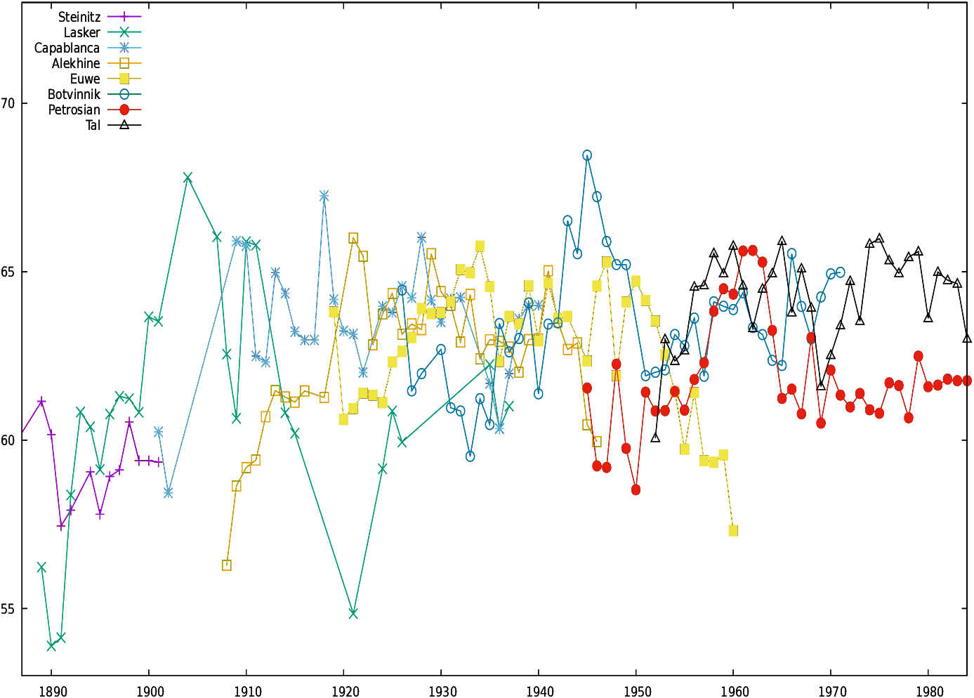
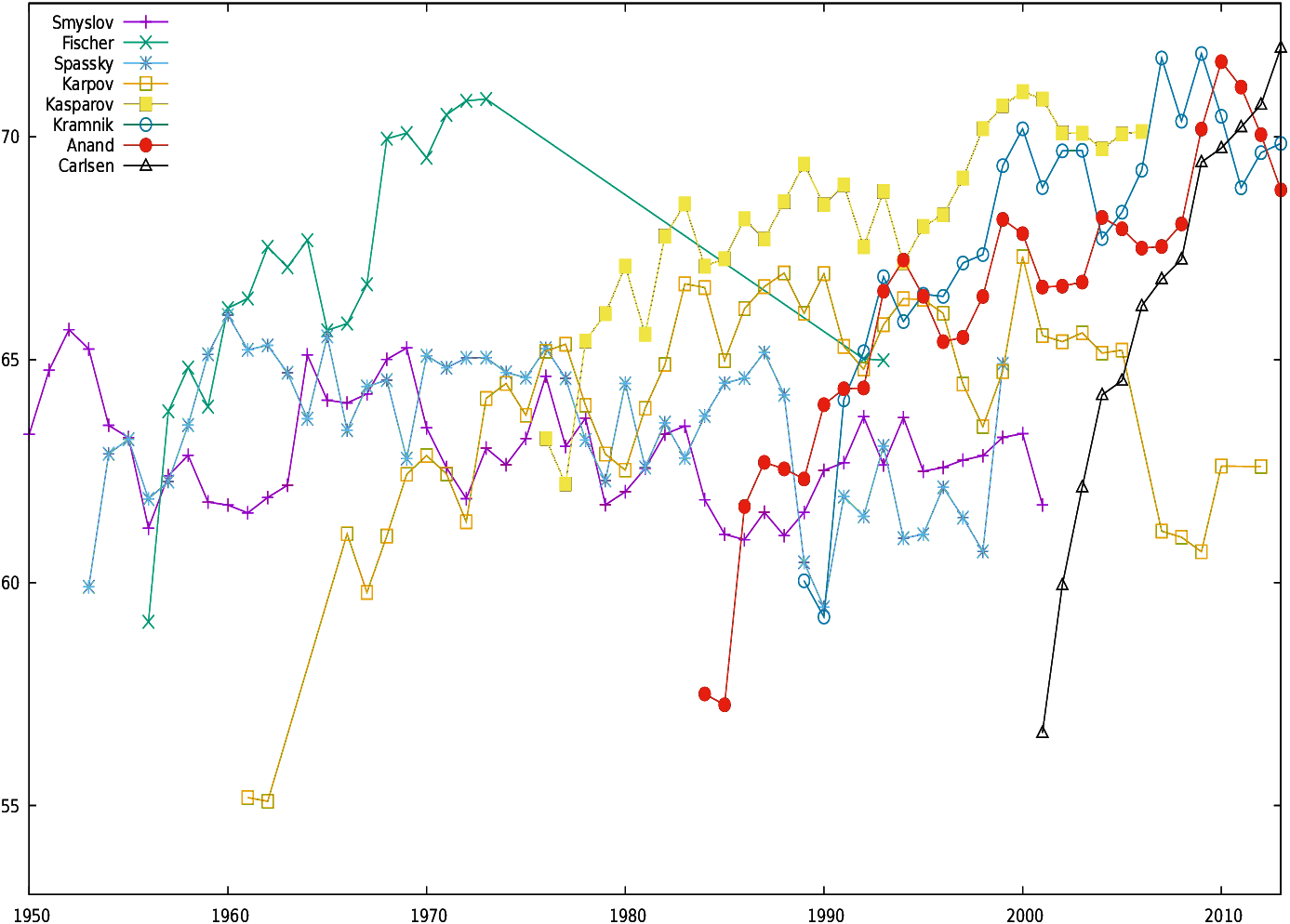
| Figure 16: Strength at 0cp |
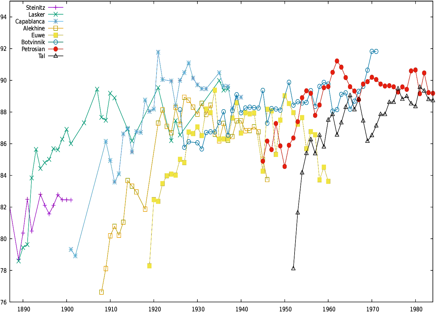
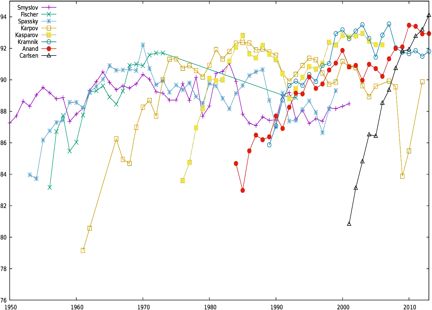
| Figure 17: Strength at 0-30cp |
This document was translated from LATEX by
HEVEA.